REVIEW 3 major objections 5 minor 40 references
Efficient Sensing of Correlated Spatiotemporal Signals: A Stochastic Gradient Approach
T0 review · 3 major / 5 minor · reviewed 2026-08-14 · deepseek-v4-flash
Pith's one-line read The paper claims that a stochastic-gradient contour-learning algorithm lets a fusion center track an unknown correlated spatiotemporal field while only about 9–10 percent of sensors report during temporal monitoring.
desk verdict Clever margin-adaptation heuristic, but the error metric measures change between successive reconstructions, not distance to the true field, so the headline efficiency claim is unverified. read the letter →
The pith
A machine-rendered reading of the paper's core claim, the machinery that carries it, and where it could break.
The reading
What carries the argument
The load-bearing object is the contour margin $\Delta$, defined as the band around each contour level $\ell_i$ such that a sensor reports only if its reading satisfies $\ell_i - \Delta \le S_k \le \ell_i + \Delta$. $\Delta$ is updated at each iteration by the normalized stochastic-gradient rule $\Delta_k = \Delta_{k-1}\left(1 + \frac{\mathrm{Error}_{k-1} - \mathrm{Error}_{k-2}}{\mathrm{Error}_{k-1} + \mathrm{Error}_{k-2}}\right)$, so the margin widens when the reconstruction error increases (admitting more sensors) and narrows when the error decreases (suppressing transmissions). Around this update the algorithm wraps Lloyd-Max contour-level selection (Eqs. 1–2), bi-harmonic spline interpolation, moving-average noise filtering, and online range and pdf estimation. Together these pieces let the fusion center learn the field's structure while using the margin as a single scalar control of the cost–fidelity trade-off.
What would settle it
Run the algorithm on the same synthetic diffusion fields and compare the metric in Eq. (3) against the error computed with respect to the known ground-truth field, especially during the temporal phase where the wider Gaussian components move horizontally; if the two error measures diverge, for example Eq. (3) stays small while the true error grows, the paper's claim that about 9–10 percent reporting preserves monitoring performance is not supported.
Extended reading notes
Core claim
The central claim is that a spatiotemporal field can be tracked by a contour-line model whose parameters are learned online rather than known beforehand, and that a well-chosen adaptive margin $\Delta$ is what makes the monitoring cheap without sacrificing reconstruction quality. Starting from a coarse range guess taken from two arbitrary sensors, the fusion center iteratively increases the number of contour levels $M$, reconstructs the field with bi-harmonic spline interpolation from reports within $\Delta$ of each level, updates the signal range from the interpolant's output, estimates the field's pdf with a Kolmogorov-Smirnov test, and adjusts $\Delta$ according to the normalized gradient of the reconstruction error given in Eq. (5). The paper shows on synthetic diffusion fields that this adaptive scheme reaches a steady state in which roughly 9–10 percent of sensors report during each temporal monitoring period, and that this reporting fraction and the reconstruction error both remain stable across iterations.
Load-bearing premise
The load-bearing premise is that the difference between one reconstruction and the next faithfully represents how accurate the monitoring is; if successive reconstructions stay similar while drifting away from the true field, the reported savings in transmissions would not prove the field is being tracked accurately.
Editorial extensions
If this is right
- A network can start monitoring a completely unknown field from just a few sensor readings and converge to a low-cost steady state without any calibration phase that assumes statistics of the field.
- Temporal tracking after convergence needs only about 9–10 percent of sensors to transmit per period, which extends battery life roughly in proportion to the reduction in transmissions.
- The margin $\Delta$ converges to a tight band from different starting values, so the algorithm does not require careful hand-tuning of the reporting threshold.
- Choosing Lloyd-Max contour levels instead of uniform levels gives reconstruction performance between fixed-level Lloyd-Max and uniform spacing while keeping the reporting cost close to the uniform scheme.
Reading between the lines
- The normalized gradient update for $\Delta$ depends only on the scalar error sequence, so the same control law could tune the sampling budget in other selective-sensing schemes, such as adaptive quantization or variable-rate compressive sensing.
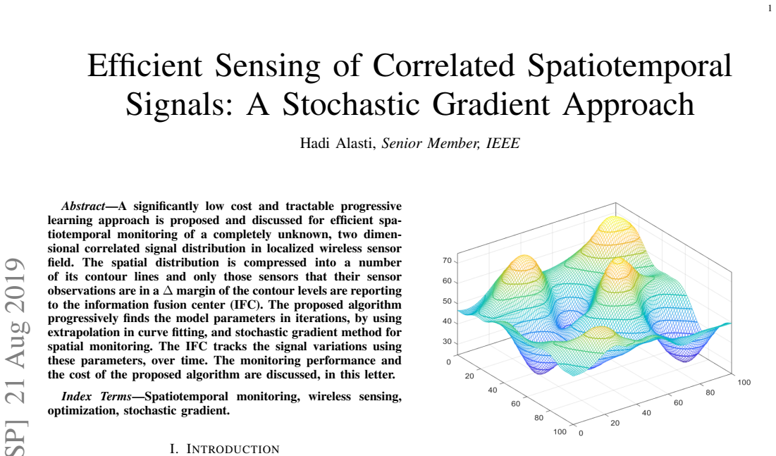
- The 9–10 percent reporting figure comes from synthetic diffusion fields with Gaussian components of standard deviation 3 and 10; fields with sharper gradients would likely require a narrower margin and a larger reporting fraction, which is a direct testable prediction.
- Because the paper's error measure is the average absolute change between successive reconstructions rather than error against a true field, the reported cost savings establish reconstruction stability; an independent ground-truth comparison would be needed to assert absolute tracking accuracy.
Signed reviews
Editorial analysis
A structured set of objections, weighed in public.
Referee Report
Summary. The paper proposes a centralized contour-based learning algorithm for spatiotemporal monitoring of an unknown two-dimensional correlated field in a wireless sensor network. Sensors whose readings fall within a margin Δ of estimated contour levels report to the IFC, which reconstructs the field using bi-harmonic spline interpolation. The algorithm progressively increases the number of contour levels, estimates the signal range and pdf, and adapts Δ through a normalized stochastic-gradient rule (Eq. (5)). For temporal monitoring, the IFC periodically queries sensors using the converged levels and margin. The paper reports that roughly 9–10% of sensors report during temporal monitoring and that the adaptive schemes outperform a fixed-margin Lloyd-Max baseline in terms of its stated error criterion.
Significance. If the claimed transmission savings were accompanied by a valid accuracy measure, the algorithm would be a useful contribution to energy-constrained field monitoring. The paper includes reproducible elements: the simulation model is explicit, the code is linked in [40], and the comparison among three contour-level schemes is a reasonable experimental design. However, the central performance claim rests on a metric that is not validated against ground truth, which prevents the results from supporting the stated efficiency and monitoring-quality claims.
major comments (3)
- [Section III-A, Eq. (3)] The quantity in Eq. (3), repeatedly called the 'mean reconstruction error,' is the mean absolute difference between successive reconstructions, not the error between a reconstruction and the true field. A reconstruction that never changes yields Error_n = 0 and would appear perfect under this metric. Therefore Figures 5 and 6, which plot this quantity, do not establish monitoring accuracy; they are also consistent with a stagnant or lagging reconstruction. Because this is the paper's only performance metric, the central claim of efficient monitoring is unsupported.
- [Section IV-B, Eq. (6)] The simulation fully knows the ground-truth field g(x,y) from Eq. (6), yet no figure compares the reconstruction g̃_n to the true field. The temporal monitoring performance in Fig. 6 swings around a value that is not ground-truth error. A direct comparison to g is necessary to validate the reported 9–10% reporting rate in Fig. 4; without it, the claimed transmission saving has no verified accuracy counterpart.
- [Section III-A, Eq. (5)] The Δ-adaptation in Eq. (5) is driven by differences in the successive-reconstruction quantity from Eq. (3). Consequently, the convergence shown in Fig. 7 demonstrates only that the adaptation stabilizes an internal statistic of the algorithm; it does not show convergence toward accurate reconstruction of the true field. The learning step is thus circular with the biased error metric, and the claim that the algorithm 'progressively finds the model parameters' is not supported by the presented evidence.
minor comments (5)
- [Section IV, Eq. (6)] The text states that σa and σb are 10 and 3, respectively, but then says the Gaussian terms with standard deviation σb = 10 are moved; Eq. (6) itself defines σb as a parameter. These statements are inconsistent and should be corrected.
- [Section III-A, Eqs. (1)-(2)] Equations (1) and (2) are incomplete because the boundary values y0 and yM that define the integration limits for the extreme contour levels are never specified.
- [Algorithm summary, Step 5] Step 5 of the algorithm summary says the IFC 'estimates the mean absolute error,' but the quantity actually computed by Eq. (3) is the mean absolute difference between successive reconstructions. The wording should be changed to avoid implying that ground-truth error is computed.
- [Section III-A, margin condition] The reporting condition is written as 'l_i - Δ ≤ S_k ≤ l_i - Δ' in Section III-A; the second sign should be '+'.
- [Section IV, Figures 3-7] No error bars, confidence intervals, or multiple independent trials are reported for the cost and error curves, making it difficult to assess the variability of the reported 9–10% reporting rate and the convergence behavior.
Circularity Check
No equation-level circularity; the new Δ-adaptation is independent, though the framework leans on the author's prior [12].
full rationale
The derivation chain is not circular by construction. The paper's contribution is the normalized-gradient Δ-adaptation in Eq. (5), driven by the internal quantity Error_n of Eq. (3); no parameter is fitted to ground truth and then reused as a prediction of that same ground truth, and the simulation results in Section IV are observations rather than identities forced by the definitions. The biggest weakness is not circularity but metric validity: Eq. (3) calls the mean absolute difference between successive reconstructions a 'signal estimation error,' so a frozen reconstruction would score zero in Figs. 5 and 6 regardless of distance to the true field; that is a correctness concern, not a circular derivation. Several references, including [12], [15], [21]-[23], [28], and [40], are self-citations, and the contour-based monitoring framework is inherited from [12] ('The proper number of contour lines and their levels are calculated in the process of spatial monitoring based on the proposed approach in [12]'), but the new Δ mechanism is independently stated and tested on synthetic data, so the self-citation chain does not force the paper's central conclusion. Score 2 reflects minor self-citation without load-bearing construction-level circularity.
Assumptions & free parameters
free parameters (4)
- Initial number of contour levels M =
3 (suggested)
- Initial contour margin Δ =
Not fixed; text says Δ = (𝓁1+𝓁2)/2, algorithm summary says Δ = (𝓁2−𝓁1)/2
- Moving average filter tap count m =
Not specified
- Number of sensors queried for initial range =
'a few (at least two)'
assumptions (5)
- domain assumption The IFC knows the coordinates of all sensors (localization).
- domain assumption The signal distribution is spatially correlated and can be approximated by a finite set of contour lines.
- domain assumption Bi-harmonic spline interpolation from samples near contour lines yields an accurate reconstruction of the field.
- ad hoc to paper The level-crossing margin adaptation (Eq. 5) converges to a suitable Δ and that the error difference Error_{k-1} - Error_{k-2} is a useful gradient signal.
- domain assumption Zero-mean Gaussian noise with power σ², reducible to σ²/m by a moving average filter whose taps do not distort the signal.
Cite this review
Pith. "Pith review of Efficient Sensing of Correlated Spatiotemporal Signals: A Stochastic Gradient Approach." pith.science (2026). https://pith.science/paper/NQ25ACKB
@misc{pith2026190807674,
  author       = {Pith},
  title        = {Pith review of: Efficient Sensing of Correlated Spatiotemporal Signals: A Stochastic Gradient Approach},
  year         = {2026},
  howpublished = {\url{https://pith.science/paper/NQ25ACKB}},
  note         = {Machine review of arXiv:1908.07674}
}
abstract
A significantly low cost and tractable progressive learning approach is proposed and discussed for efficient spatiotemporal monitoring of a completely unknown, two dimensional correlated signal distribution in localized wireless sensor field. The spatial distribution is compressed into a number of its contour lines and only those sensors that their sensor observations are in a $\Delta$ margin of the contour levels are reporting to the information fusion center (IFC). The proposed algorithm progressively finds the model parameters in iterations, by using extrapolation in curve fitting, and stochastic gradient method for spatial monitoring. The IFC tracks the signal variations using these parameters, over time. The monitoring performance and the cost of the proposed algorithm are discussed, in this letter.
Figures


Figures from the paper (3 more)


Reference graph
Works this paper leans on
-
[40]
Alasti, (2019) Efficient spatiotemporal monitoring of correlated signals based on stochastic gradient [Online]
H. Alasti, (2019) Efficient spatiotemporal monitoring of correlated signals based on stochastic gradient [Online]. Available: https://github.com/HarryAlasti/Stochastic-Gradient-Spatiotemporal- Monitoring
2019
- [1]
-
[2]
M.C. Vuran, O.B. Akan and I.F. Akyildiz, Spatio-temporal correlation: theory and applications for wireless sensor networks, in Computer Networks vol.45, no.3, p.245-259, June 2004
work page 2004
-
[3]
A. Kramer and T.A. Paul, High-precision density sensor for concentra- tion monitoring of binary gas mixtures, in Proceedings of Eurosensors XXVI, p. 44-47, September 9-12, 2012, Krakw, Poland
work page 2012
-
[4]
J.-H. Liu, Y .-F. Chen, An air quality monitoring system for urban areas based on the technology of wireless sensor networks, Internatinal Journal on Smart Sensing and Intelligent Systems, vol. 5, no. 1, Mar 2012
work page 2012
-
[5]
Y . Zhao, B. Huang, Integrating modis and MTSAT-2 to generate high spatial-temporal-spectral resolution imagery for real-time air quality monitoring, IEEE International Geoscience and Remote Sensing Sym- posium (IGARSS), p. 6122 - 6125, 2017
work page 2017
- [6]
- [7]
Show all 40 references
-
[8]
Akyildiz, W
I.F. Akyildiz, W. Su, Y . Sankarasubramanuam, E. Cayirci, Wireless sensor networks: a survey, Computer Networks, vol. 38, pp. 393-422, December 2002
2002
-
[9]
Costilla-Reyes, P
O. Costilla-Reyes, P. Scully, K.B. Ozanyan, Deep neural networks for learning spatio-temporal features from tomography sensors, IEEE Transactions on Industrial Electronics, p. 645-653, vol. 65, no. 1, 2018
2018
-
[10]
Gokaraju, S.S
B. Gokaraju, S.S. Durbha, R.L. King, N.H. Younan A machine learning based spatio-temporal data mining approach for detection of harmful algal blooms in the gulf of mexico, in IEEE Journal of selected Topics in Applied Earth Observations and Remote Sensing, p. 710-720, vol. 3, ...
2011
-
[11]
Zhang, I
P. Zhang, I. Nevat, G.W. Peters, F. Septier, M.A. Osborne, Spatial field reconstruction and sensor selection in heterogeneous sensor networks with stochastic energy harvesting, IEEE Transactions on Signal Pro- cessing, V ol.66, no.9, p.2245 - 2257, 2018
2018
-
[12]
H. Alasti, An on-demand compressed sensing approach for spatial monitoring of correlated big data using multi-contours in dense wireless sensor network, in proceedings of IEEE International Conference on Wireless for Space and Extreme Environments (WiSEE), p. 86-91, Montreal, 2017
2017
-
[13]
Barcel-Llad, A
J.E. Barcel-Llad, A. Morell, G. Seco-Granados, Amplify-and-forward compressed sensing as an energy-efficient solution in wireless sensor networks, IEEE Sensors Journal, V ol.14, no.5, p.1710 - 1719, 2014
2014
-
[14]
H. Alasti, Level based sampling techniques for energy conservation in large scale wireless sensor networks, Unpublished doctoral dissertation, University of North Carolina, Charlotte, 2009
2009
-
[15]
Alasti, A
H. Alasti, A. Nasipuri, Spatiotemporal monitoring using contours in Large-scale wireless sensor networks, ACM FOW ANC09, May 18, pp. 77-85, 2009, New Orleans, Louisiana, USA
2009
-
[16]
Marvasti, Nonuniform Sampling, Kluwer Academic, 2001
F. Marvasti, Nonuniform Sampling, Kluwer Academic, 2001
2001
-
[17]
Guan, S.S
K.M. Guan, S.S. Kozat, A.C. Singer, Adaptive reference levels in a level- crossing analog-to-digital converter, EURASIP Journal on Advances in Signal Processing vol. 2008, Jan. 2008
2008
-
[18]
Candes, Compressive sampling, in Proc
E.J. Candes, Compressive sampling, in Proc. IEEE Intl. Congress of Mathematicians, Madrid, Spain, 2006
2006
-
[19]
Donoho, Compressed sensing, in IEEE Transactions on Information Theory, vol.52, no.4, pp.1289-1306, April 2006
D. Donoho, Compressed sensing, in IEEE Transactions on Information Theory, vol.52, no.4, pp.1289-1306, April 2006
2006
-
[20]
S. Li, L.D. Xu, X. Wang, Compressed Sensing Signal and Data Acquisition in Wireless Sensor Networks and Internet of Things, IEEE Trans. on Industrial Informatics, vol.9,no.4, Nov. 2013
2013
-
[21]
Alasti, Non-uniform-level crossing sampling for efficient sensing of temporally sparse signals , IET Wireless sensor systems, vol
H. Alasti, Non-uniform-level crossing sampling for efficient sensing of temporally sparse signals , IET Wireless sensor systems, vol. 4, no. 1, pp. 27-34, 2014
2014
-
[22]
H. Alasti, Level crossing sampling for energy conservation in wireless sensor networks: A design framework, , book chapter in Wireless Tech- nologies: Concepts, Methodologies, Tools and Applications, IGI Global, 2011
2011
-
[23]
Alasti, Energy efficient spatiotemporal threshold level detection in large scale wireless sensor fields, IEEE Online Conference on Green Communications (GreenCom), pp
H. Alasti, Energy efficient spatiotemporal threshold level detection in large scale wireless sensor fields, IEEE Online Conference on Green Communications (GreenCom), pp. 151-156, 2012
2012
-
[24]
Liao, M.K
P.K. Liao, M.K. Chang, C.C.J. Kuo, Contour line extraction in a multi- modal field with sensor networks, Proceedings IEEE Global Telecom- munication Conference (Globecom), 2005
2005
-
[25]
Liao, M.K
P.K. Liao, M.K. Chang, C.C.J. Kuo, A distributed approach to contour line extraction using sensor networks, in Proc. IEEE VTC, 2005
2005
-
[26]
Liao, M.K
P.K. Liao, M.K. Chang, C.C.J. Kuo, Contour line extraction with wireless sensor networks, in Proc. IEEE International Conference on Communications (ICC), 2005
2005
-
[27]
Liao, M.K
P.K. Liao, M.K. Chang, C.C.J. Kuo, A cross-layer approach to contour nodes inference with data fusion in wireless sensor networks, in the Proceedings of Wireless Communications and Networking Conference (IEEE WCNC’07) pages 2773-2777, 2007
2007
-
[28]
Alasti, W.A
H. Alasti, W.A. Armstrong, A. Nasipuri, Performance of a robust filter- based approach for contour detection in wireless sensor networks, in Proceedings of ICCCN’07, pages 159-164, 2007
2007
-
[29]
Buragohain, S
C. Buragohain, S. Gandhi, J. Hershberger, S. Suri, Contour approxima- tion in sensor networks, DCOSS ’06, June 18-20, 2006
2006
-
[30]
Gandhi, J
S. Gandhi, J. Hershberger, S. Suri, Approximate iso-contours and spatial summaries in sensor networks, IPSN’07, April 25-27, 2007
2007
-
[31]
Sarkar, X
R. Sarkar, X. Zhu, J. Gao, L.J. Guibas, J.S.B. Mitchell, Iso-contour queries and gradient descent with guaranteed delivery in sensor net- works, in Proceedings of IEEE INFOCOM’08, 2008
2008
-
[32]
J. Lian, L. Chen, K. Naik, Y . Liu, G.B. Agnew, Gradient boundary detection for time series snapshot construction in sensor networks, IEEE Transactions on Parallel and Distributed Systems, vol.18, no.10, pp. 1462-1475, Oct. 2007
2007
-
[33]
W. Dai, Y . Shen, H. Xiong, X. Jiang, J. Zou, D. Taubman, Progressive dictionary learning with hierarchical predictive structure for low bit- rate scalable video coding, in IEEE Transactions on Image Processing, p. 2972-2987, vol. 26, no. 6, 2017
2017
-
[34]
Sandwell, Bipolar spline interpolation of GEOS-3 and SEASAT altimeter data, Geophysical Research Letters, vol
D.T. Sandwell, Bipolar spline interpolation of GEOS-3 and SEASAT altimeter data, Geophysical Research Letters, vol. 14, no. 3, pp. 139- 142, Feb. 1987
1987
-
[35]
Sayood, Introduction to data compression, Published by Morgan Kaufmann, 2000
K. Sayood, Introduction to data compression, Published by Morgan Kaufmann, 2000
2000
-
[36]
Bershad, Analysis of the normalized LMS algorithm with Gaussian inputs, in IEEE Transactions on Acoustics, Speech, and Signal Process- ing, p
N. Bershad, Analysis of the normalized LMS algorithm with Gaussian inputs, in IEEE Transactions on Acoustics, Speech, and Signal Process- ing, p. 793-706, vol. 34, no. 4,1986
1986
-
[37]
Conover, Practical nonparametric statistical, 3rd edition, pp.428- 433, John Wiley & Sons, Inc
W.J. Conover, Practical nonparametric statistical, 3rd edition, pp.428- 433, John Wiley & Sons, Inc. New York, 1999
1999
-
[38]
Jindal, K
A. Jindal, K. Psounis, Modeling spatially-correlated data of sensor networks with irregular topologies, in Proceedings of IEEE International Conference on Sensor and Ad hoc Communications and Networks (SECON’05), Santa Clara, CA, September 2005
2005
-
[39]
Jindal, K
A. Jindal, K. Psounis, Modeling spatially correlated data in sensor networks, ACM Transactions on Sensor Networks, November 2006
2006
Reviewed August 14, 2026 · model on record in the stance chip above.
Discussion (0). Continue with ORCID to comment.