Extension to mixed models of the Supervised Component-based Generalised Linear Regression

Catherine Trottier (IMAG; Frederic Mortier (UPR 105 BSEF); Jocelyn Chauvet (IMAG); UM3); Xavier Bry (IMAG)

REVIEW 4 major objections 6 minor 10 references

Extension to mixed models of the Supervised Component-based Generalised Linear Regression

T0 review · 4 major / 6 minor · reviewed 2026-08-14 · deepseek-v4-flash

Challenge this review Re-run · record.json Download PDF Read on arXiv ↗ Review JSON

Pith's one-line read The paper extends the SCGLR component-based regularisation criterion to generalized linear mixed models, claiming lower mean relative error than Ridge or Lasso on grouped data with redundant predictors and interpretable components on a…

desk verdict A coherent and genuinely new extension of SCGLR to GLMMs via Schall's algorithm, but the empirical case only covers the Gaussian regime and the simulation metric flatters single-response fits. read the letter →

arxiv 1908.07908 v1 pith:NQS2BNXT submitted 2019-08-09 stat.ME

Jocelyn Chauvet (IMAG) , Catherine Trottier (IMAG , UM3) , Xavier Bry (IMAG) , Frederic Mortier (UPR 105 BSEF) This is my paper · ORCID

classification stat.ME MSC 62J1262J07

keywords component-basedregularisationmultivariateGLMMrandomeffectsstructuralrelevanceSCGLRSchall'salgorithmHendersonequationsRidge-Lassocomparison

verification ladder T0 review T1 audit T2 compute T3 formal

The pith

A machine-rendered reading of the paper's core claim, the machinery that carries it, and where it could break.

The reading

Mixed-SCGLR extends the Supervised Component-based Generalised Linear Regression (SCGLR) to generalized linear mixed models, so that data with grouped or correlated units and many redundant predictor variables can be analysed without collapsing the dependence structure. The method alternates between building an orthogonal component $f=Xu$ that balances fit to the responses (through Schall's working variables) with proximity to the strongest directions in $X$, and estimating fixed and random effects from Henderson systems. The paper's simulations indicate that, when the predictors contain genuine latent bundles, this component-based regularisation has lower mean relative error than Ridge or Lasso-regularised mixed models; on a Poisson count dataset of tree genera, it selects components that separate rainfall/wind and photosynthesis signals. A sympathetic reader would take the contribution to be a practical, interpretable alternative to penalty-based regularisation for multivariate GLMMs.

What carries the argument

The optimization problem at the heart of the method is $$\max_{u'Au=1}\,[\varphi(u)]^s[\psi_T(u)]^{1-s},$$ where $f=Xu$ is a component, $\varphi(u)$ measures how close $Xu$ is to the strongest structures in $X$ (a sum over variables of powered correlations), and $\psi_T(u)$ measures how well $Xu$ plus the extra covariates $T$ explains Schall's working variables $z_{\xi}^k$ in the weighted metric $W_{\xi,k}$. Conditional on $u$, the fixed effects $\gamma_k$, $\delta_k$ and random effects $\xi_k$ are obtained by solving the Henderson system (5), and the variance parameters $\sigma_k^2$ are updated by Schall's formula. The Projected Iterated Normed Gradient (PING) algorithm maximizes the criterion on the sphere $u'Au=1$ under orthogonality constraints when building higher-rank components.

What would settle it

Replicate the Section 4 simulation with Poisson or binomial responses, small groups (e.g., N=10 groups of size 5), and known coefficient vectors; compute the mean relative error for Mixed-SCGLR, LMM-Ridge and (G)LMM-Lasso with cross-validated tuning. If for $\tau\ge0.3$ Mixed-SCGLR is not at least as accurate as the best penalised alternative, the claim that it performs well on grouped data would be contradicted; a second check is whether the maximised criterion in Equation (3) increases monotonically along the PING iterations, since a non-monotone path indicates possible local-maximum stops.

Watch

Extended reading notes

Core claim

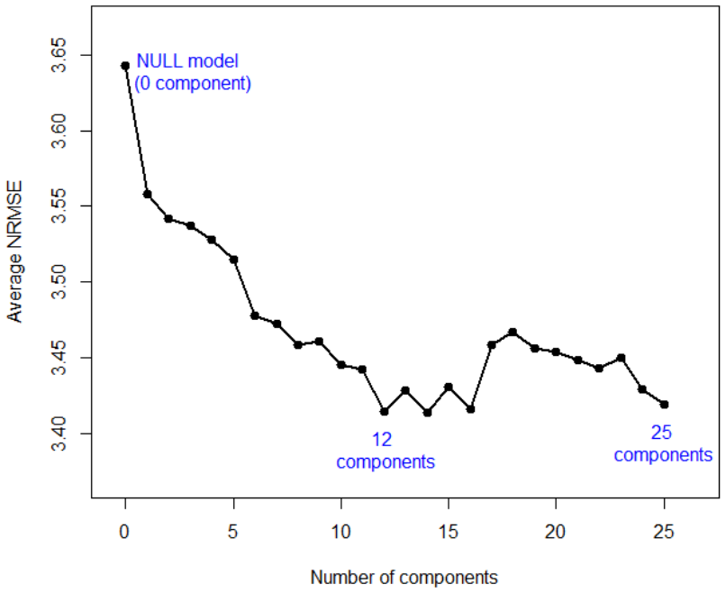
The central claim is that the SCGLR trade-off criterion, $$\max_{u'Au=1}[\varphi(u)]^s[\psi_T(u)]^{1-s},$$ can be embedded into Schall's algorithm for GLMMs, with $\psi_T$ redefined using the conditional working-variable variance $W_{\xi,k}$, and with fixed and random effects solved by Henderson systems. The paper argues that this yields a valid estimation scheme because, conditionally on the random effects, the working variables form a normal hierarchy whose posterior mode is exactly the Henderson solution, and the variance components can be updated by Schall's formula. In the Gaussian simulation, the resulting estimates are more precise than LMM-Ridge and (G)LMM-Lasso whenever the explanatory variables form strong bundles ($\tau\ge0.3$); in the Poisson example, the method produces 12 components that can be read as interpretable environmental bundles while maintaining predictive accuracy.

Load-bearing premise

The load-bearing premise is that Schall's working variables are exactly Gaussian, with the covariance the algorithm uses, conditional on the random effects; for Poisson or binomial responses with small groups this is an approximation, and every parameter update in Algorithm 1 depends on it.

Editorial extensions

If this is right

For grouped data with many redundant predictors, users can obtain a regularised multivariate GLMM without choosing a shrinkage parameter; instead they choose the number of components $K$ and the balance $s$ by cross-validation.
Because the component is common to all responses, the method borrows information across $q$ outcomes when detecting structure, unlike separate ridge or lasso fits.
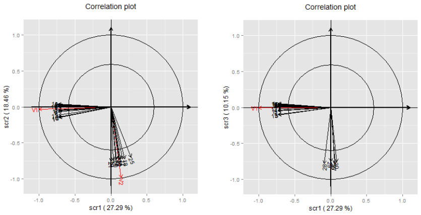
The estimated components provide a low-dimensional projection of $X$ that can be inspected through correlation scatterplots, revealing which original variables form each bundle.
On the Genus data, 12 components suffice to approximate the abundance of 94 tree genera, showing the method scales to many responses and dozens of predictors.
The inclusion of unregularised covariates $T$ means known relevant variables can be forced into the model while $X$ is still regularised by components.

Reading between the lines

Editorial extensions of the paper, not claims the author makes directly.

If the Gaussian working-variable approximation holds poorly for small groups, the Henderson step may yield biased random-effect and variance estimates; a residual or bootstrap diagnostic of Equation (7) would be a natural next check, but the paper does not provide one.
The same alternating scheme could accommodate spatial, nested or crossed random effects by changing $U$ and $A_k$; the component-building step would be unchanged.
For count data with overdispersion, adding an extra dispersion parameter would likely improve predictive intervals and may alter the selected number of components; this is an extension the paper leaves implicit.
For nearly unstructured predictors, component-based regularisation offers little advantage over a lasso, so a data-dependent choice of $s$ could recover accuracy in that regime.

Share X Bluesky LinkedIn Reddit HN

Signed reviews

No signed human review yet.

Editorial analysis

A structured set of objections, weighed in public.

Desk editor's note, referee report, and a circularity audit.

Desk Editor's Note

read the letter

The thing to know: this paper does what it says on the tin. It extends SCGLR to grouped data by embedding the component criterion in Schall's pseudo-likelihood, and the derivation is coherent. The Henderson systems, the variance updates, and the PING algorithm in the appendix all hang together. That is real work, and it is a natural extension not in the cited literature.

What is new: the combination of SCGLR's component search with Schall's working variables and REML-type variance updates. The criterion [φ(u)]^s [ψ_T(u)]^{1-s} is inherited from earlier SCGLR papers, but using the Schall working variables in ψ_T is the novel step. The paper also gives a clear algorithmic recipe (Algorithm 1) and a useful constrained optimization appendix. The real-data application to tree genus counts is a nice demonstration of interpretable components from a Poisson GLMM.

Now the soft spots, in proportion. The stress-test is right: Section 4 is the only simulation study and it is strictly Gaussian (LMM, identity link), where Equation (7)'s normal working-variable assumption holds exactly. So Table 2 can support a claim about LMMs but not about the "Generalized" part of GLMMs. The conclusion's claim that Mixed-SCGLR "performs well on grouped data" is therefore too strong. This is a load-bearing gap, not a minor one.

The simulation metric is also weak. MLRE takes the minimum relative error over the two responses for each method. That lets a method that fits one response well and ignores the other score highly. For a multivariate method, a joint error metric (e.g., sum or average, or a multivariate loss) is needed. There are also no error bars despite 500 simulations; standard errors would be trivial to add.

The real-data section has no comparison with ridge, lasso, or a standard GLMM fit, so we learn only that the method runs and gives interpretable components. Tuning is also done with some hindsight: l and s are chosen for interpretability before K is cross-validated. That is not fatal, but it should be reported as a sensitivity analysis, not as a clean selection procedure.

No code or data are provided. For an algorithmic paper in 2019, that is a real deficiency, especially because SCGLR has an R package and this extension could be implemented on top of it.

On circularity: the reader's circularity burden score of 2 is right. The estimation is not circular; components are built from current working responses and parameters are updated from the resulting Henderson systems. Cross-validation for K and s is model selection, not circular reasoning.

Who this is for: applied statisticians in ecology and biometrics who want regularized, interpretable multivariate GLMMs. They will get a useful algorithm, but they should not trust the performance claims until the non-Gaussian simulations and a fair metric show up.

Recommendation: this deserves peer review. Send it to a serious referee. The method is sound enough to be worth the referee's time, but the revision must add non-Gaussian simulations, a proper multivariate error metric with uncertainty, and ideally a public implementation.

My verdict: conditional accept, in spirit.

Referee Report

4 major / 6 minor

Summary. The manuscript proposes Mixed-SCGLR, an extension of Supervised Component-based Generalised Linear Regression to multivariate GLMMs. The method constructs orthogonal components f = Xu of the redundant X block by maximizing [φ(u)]^s [ψ_T(u)]^{1-s}, where φ measures structural relevance and ψ_T is a goodness-of-fit term built from Schall's working variables and their conditional covariance; parameters are then updated by solving Henderson systems, with variance components updated by Schall's REML-type formula. A simulation study in the Gaussian LMM setting compares Mixed-SCGLR with Ridge and Lasso regularizations, and a Poisson real-data application is presented.

Significance. If the empirical claims held, Mixed-SCGLR would offer a useful alternative to penalized methods for multivariate GLMMs with many redundant regressors, with interpretable components and few tuning parameters. The paper's formal contribution is clear: Lemma 1 gives a compact Bayesian justification of the Henderson systems, the PING algorithm in the appendix provides a concrete constrained-optimization procedure, and the extension to higher-rank components is carefully specified. However, the current evidence is weakened by the simulation metric and by the absence of a validated non-Gaussian case, so the contribution is not yet established.

major comments (4)

[Section 4, MLRE definition and Table 2] The MLRE criterion takes, for each simulation, the minimum relative error over the two responses for each method. A method that fits only one of the two responses well and the other poorly will obtain the same low score as a method that fits both moderately, so Table 2 does not support the claim that Mixed-SCGLR gives more precise fixed-effect estimates than Ridge or Lasso. Please report per-response relative errors, with standard errors or quantiles over the 500 simulations, and use a joint or average criterion that rewards balanced multivariate performance.
[Sections 3.1 and 5, Eq. (7)] Equation (7) states that Schall's working variables z_ξ^k are exactly Gaussian with mean (Xu)γ_k + Tδ_k + Uξ_k and covariance W^{-1}_{ξ,k}. For non-Gaussian responses this is an approximation; nevertheless every step of Algorithm 1 (Step 1's ψ_T, Step 2's Henderson system, Step 3's variance update) is derived from this Gaussian hierarchy. Section 4 simulates only linear mixed models with normal errors and identity link, where Eq. (7) holds exactly, and the Poisson analysis in Section 5 is not benchmarked against Ridge, Lasso, or a standard GLMM fit. The paper therefore provides no empirical support for the claimed performance in the generalized-linear regime.
[Section 5, tuning of l and s] The tuning parameters l=4 and s=0.5 are selected 'among a series of parameter choices' for interpretability before K is cross-validated. This order of selection can bias the reported AveNRMSE, because the same data are used to choose l and s and then to evaluate models. Please describe how l and s were chosen (e.g., on a separate tuning set) or provide a sensitivity analysis showing that the AveNRMSE conclusions are stable to reasonable changes in l and s.
[Section 3.1 and Algorithm 1] Algorithm 1 is an alternating procedure, but the stopping rule is only described as 'repeated until stability of u and parameters'; no convergence criterion or assessment is given. Since the objective changes at each iteration through the working variables, it would be useful to specify a precise stopping tolerance and to report convergence behavior or failures in the simulations.

minor comments (6)

[Section 1] There are several typos in the introduction, for example 'developped' should be 'developed' and 'unknow' should be 'unknown'.
[Tables 1 and 2] The notation 'Mixed-SC(G)LR' is inconsistent with 'Mixed-SCGLR' used in the rest of the paper; please unify the notation.
[Section 3.2, Eq. (9)] In the definition of D_h = X' W F_h, the metric W is not specified; it should be stated whether W is the same as in Eq. (2) or a response-weighted metric.
[Section 4, Table 1] Table 1 reports optimal parameter values but not their variability over the 500 simulations; adding standard deviations or an interquartile range would strengthen the comparison.
[Figure 2 caption] The caption refers to 'X-part linear predictors' as supplementary variables, but this term is not defined before the figure; please clarify.
[Section 5] The text contains 'developped plots' and 'parcimonious'; these should be 'developed plots' and 'parsimonious'.

Circularity Check

0 steps flagged · score 0.0 of 10

No circularity: Mixed-SCGLR iteratively builds components from X and current Schall working responses and solves Henderson systems; self-citations are not load-bearing.

full rationale

The derivation chain is self-contained. The component u is defined by maximizing [phi(u)]^s [psi_T(u)]^(1-s), where phi measures structural relevance of X alone and psi_T is a goodness-of-fit to Schall working variables; neither quantity is defined in terms of the coefficients being estimated, and the algorithm alternates between building components, solving Henderson systems, and updating variance parameters. No equation computes a target from the very values it is supposed to predict. The simulation comparison is against external Lasso/Ridge benchmarks after cross-validation, which is model selection rather than a disguised fit. The self-citations are not load-bearing: [2] supplies the SCGLR criterion restated in the paper, and [8] only recommends l=4 as a tuning value. The real caveat is external validity, not circularity: Section 4 validates the Gaussian LMM case where Eq. (7) is exact, while Section 5's Poisson example lacks a comparator, so the Section 6 claim that Mixed-SCGLR 'performs well on grouped data' is broader than the evidence. That is a correctness/evidence concern, not a circularity.

Assumptions & free parameters 4 free parameters · 6 assumptions · 0 invented entities

The central algorithm depends on a sequence of modeling choices: normal independent random effects, exponential-family conditional distributions, the Schall Gaussian approximation for working variables, a shared component across responses, and unpenalized T. In addition, s, l, K are free tuning choices selected by CV or informal search. No new physical entities are introduced.

free parameters (4)

s = 0.51-0.53 in simulations; 0.5 in real data
Weight balancing structural relevance φ and goodness of fit ψ in Eq (3); selected by cross-validation in Section 4 and by informal search in Section 5.
l = 4
Exponent in the structural-relevance criterion φ (Eq. 2) controlling local versus global variable bundles; chosen as recommended in [8] and confirmed by interpretability in Section 5.
K = 25, 5, 3, 2, 2 for τ=0.1..0.9 in Section 4; 12 in Section 5
Number of orthogonal components; selected by cross-validation (Table 1, Figure 3). It is a model dimension, not derived.
Metric matrix A = unspecified
The identifiability constraint u'Au=1 in Eqs (1)-(3) depends on an arbitrary symmetric positive definite A; the paper never defines A, leaving a free choice that affects the solution.

assumptions (6)

domain assumption Random effects ξ_1,...,ξ_q are independent and normally distributed as N_N(0, σ²_k A_k), with A_k known (often I_N).
Section 3.1 states this; it is the basis for the Bayesian posterior derivation of the Henderson system. The normality is not validated in the applications.
domain assumption Conditional on random effects, each response Y_k follows a distribution in the exponential family.
Section 3.1 writes the conditional density in exponential-family form; this is the standard GLMM framework.
ad hoc to paper Working variables z_ξ^k are exactly Gaussian conditional on random effects, as in Equation (7).
This is Schall's approximation and is not exact for non-Gaussian GLMMs; all Henderson-system updates rely on it.
domain assumption The additional covariates T are few and selected so as to require no regularization.
Section 1 assumes it; if T is high-dimensional or collinear, the unpenalized treatment breaks down.
domain assumption A single component f = Xu is common to all q responses at each extraction step.
Section 1 and Eq (4) impose this shared-structure assumption; it is the defining modeling choice of SCGLR.
standard math Improper noninformative priors are used for fixed-effect coefficients γ_k and δ_k (Bγ^{-1}=Bδ^{-1}=0).
Section 3.1 adopts this from Stiratelli et al.; it is a standard Bayesian device, not a data-driven choice.

how reviews work

0 comments

Cite this review

Pith. "Pith review of Extension to mixed models of the Supervised Component-based Generalised Linear Regression." pith.science (2026). https://pith.science/paper/NQS2BNXT

@misc{pith2026190807908,
  author       = {Pith},
  title        = {Pith review of: Extension to mixed models of the Supervised Component-based Generalised Linear Regression},
  year         = {2026},
  howpublished = {\url{https://pith.science/paper/NQS2BNXT}},
  note         = {Machine review of arXiv:1908.07908}
}

read the original abstract

We address the component-based regularisation of a multivariate Generalized Linear Mixed Model (GLMM). A set of random responses Y is modelled by a GLMM, using a set X of explanatory variables, a set T of additional covariates, and random effects used to introduce the dependence between statistical units. Variables in X are assumed many and redundant, so that regression demands regularisation. By contrast, variables in T are assumed few and selected so as to require no regularisation. Regularisation is performed building an appropriate number of orthogonal components that both contribute to model Y and capture relevant structural information in X. To estimate the model, we propose to maximise a criterion specific to the Supervised Component-based Generalised Linear Regression (SCGLR) within an adaptation of Schall's algorithm. This extension of SCGLR is tested on both simulated and real data, and compared to Ridge- and Lasso-based regularisations.

Figures

Figures reproduced from arXiv: 1908.07908 by the authors.

**Figure 1.** Polar representation of φ l (u) according to the value of l, in the elementary case of four coplanar variables. Principle We maintain predictors colinear in their X-parts. Introducing a random effect in each predictor and still imposing u 0Au = 1, the linear predictors now write: ∀k ∈ {1, . . . , q} , ηk ξ = (Xu)γk + T δk + Uξk (4) The random group effect is assumed different accross responses, yielding q random eff… view at source ↗

**Figure 2.** Correlation scatterplots given by Mixed-SCGLR method on the simulated data. [PITH_FULL_IMAGE:figures/full_fig_p009_2.png] view at source ↗

**Figure 3.** AveNRMSE’s as a function of the number of components, obtained by a cross [PITH_FULL_IMAGE:figures/full_fig_p010_3.png] view at source ↗

Figures from the paper (1 more)

**Figure 4.** Figure 4: Two examples of correlations scatterplots on data [PITH_FULL_IMAGE:figures/full_fig_p011_4.png]

Discussion (0). Continue with ORCID to comment.

Reference graph

Works this paper leans on

10 extracted references · 10 canonical work pages

[1]

and Tenenhaus, M

Bastien, P., Esposito Vinzi, V. and Tenenhaus, M. (2004) PLS generalized linear regression. Computational Statistics & Data Analysis, 48, 17–46

work page 2004
[2]

and Mortier, F

Bry, X., Trottier, C., Verron, T. and Mortier, F. (2013) Supervised component gener- alized linear regression using a PLS-extension of the Fisher scoring algorithm. Journal of Multivariate Analysis, 119, 47-60

work page 2013
[3]

and Foulkes, A.S

Eliot, M., Ferguson, J., Reilly, M.P. and Foulkes, A.S. (2011) Ridge Regression for Longitudinal Biomarker Data. The International Journal of Biostatistics, 7, 1–11

work page 2011
[4]

and Tutz, G

Groll, A. and Tutz, G. (2014) Variable Selection for Generalized Linear Mixed Models by L1-Penalized Estimation. Statistics and Computing, 24, 137–154

work page 2014
[5]

(1975) Best linear unbiaised estimators and prediction under a se- lection model

Henderson, C.R. (1975) Best linear unbiaised estimators and prediction under a se- lection model. Biometrics, 31, 423-447

work page 1975
[6]

(1996) Iteratively reweighted partial least squares estimation for general- ized linear regression

Marx, B.D. (1996) Iteratively reweighted partial least squares estimation for general- ized linear regression. Technometrics, 38, 374-381

work page 1996
[7]

and Searle, S.R (2001) Generalized, Linear, and Mixed Models

McCulloch, C.E. and Searle, S.R (2001) Generalized, Linear, and Mixed Models. John Wiley & Sons

work page 2001
[8]

(2015) SCGLR - An R Package for Supervised Component Generalized Linear Regression

Mortier, F., Trottier, C., Cornu, G., Bry, X. (2015) SCGLR - An R Package for Supervised Component Generalized Linear Regression

work page 2015

Show all 10 references

[9]

(1991) Estimation in generalized linear models with random eﬀects

Schall, R. (1991) Estimation in generalized linear models with random eﬀects. Biometrika, 78, 719-727

1991
[10]

(1984) Random-Eﬀects Models for Serial Observations with Binary Response

Stiratelli, R., Laird, N., and Ware, J.H. (1984) Random-Eﬀects Models for Serial Observations with Binary Response. Biometrics, 40, 961–971. 12

1984

Pith tools

Reviewed August 14, 2026 · model on record in the stance chip above.

[1] [1]

and Tenenhaus, M

Bastien, P., Esposito Vinzi, V. and Tenenhaus, M. (2004) PLS generalized linear regression. Computational Statistics & Data Analysis, 48, 17–46

work page 2004

[2] [2]

and Mortier, F

Bry, X., Trottier, C., Verron, T. and Mortier, F. (2013) Supervised component gener- alized linear regression using a PLS-extension of the Fisher scoring algorithm. Journal of Multivariate Analysis, 119, 47-60

work page 2013

[3] [3]

and Foulkes, A.S

Eliot, M., Ferguson, J., Reilly, M.P. and Foulkes, A.S. (2011) Ridge Regression for Longitudinal Biomarker Data. The International Journal of Biostatistics, 7, 1–11

work page 2011

[4] [4]

and Tutz, G

Groll, A. and Tutz, G. (2014) Variable Selection for Generalized Linear Mixed Models by L1-Penalized Estimation. Statistics and Computing, 24, 137–154

work page 2014

[5] [5]

(1975) Best linear unbiaised estimators and prediction under a se- lection model

Henderson, C.R. (1975) Best linear unbiaised estimators and prediction under a se- lection model. Biometrics, 31, 423-447

work page 1975

[6] [6]

(1996) Iteratively reweighted partial least squares estimation for general- ized linear regression

Marx, B.D. (1996) Iteratively reweighted partial least squares estimation for general- ized linear regression. Technometrics, 38, 374-381

work page 1996

[7] [7]

and Searle, S.R (2001) Generalized, Linear, and Mixed Models

McCulloch, C.E. and Searle, S.R (2001) Generalized, Linear, and Mixed Models. John Wiley & Sons

work page 2001

[8] [8]

(2015) SCGLR - An R Package for Supervised Component Generalized Linear Regression

Mortier, F., Trottier, C., Cornu, G., Bry, X. (2015) SCGLR - An R Package for Supervised Component Generalized Linear Regression

work page 2015