REVIEW 4 major objections 4 minor 50 references
Constrained Thompson Sampling for Real-Time Electricity Pricing with Grid Reliability Constraints
T0 review · 4 major / 4 minor · reviewed 2026-08-14 · deepseek-v4-flash
Pith's one-line read The paper proves that a constrained Thompson sampling algorithm can learn real-time electricity prices while keeping distribution-system voltage and line-flow limits intact, with a logarithmic regret bound.
desk verdict A genuinely useful constrained-TS formulation whose safety guarantee is currently unsupported: Assumption 4 as printed is impossible and inequality (19) is cited, not proved. read the letter →
The pith
A machine-rendered reading of the paper's core claim, the machinery that carries it, and where it could break.
The reading
What carries the argument
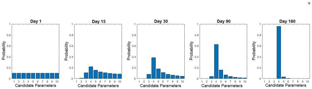
The load-bearing object is the posterior-mass floor $\pi_\tau(\theta^\star) \ge \pi_0(\theta^\star)e^{-\lambda|\mathcal{P}|}$, carried over from the Bayesian analysis of Thompson sampling for complex online problems. Combined with the posterior-averaged chance constraints (16)-(18), this floor converts a belief about the customer model into a statement about the true model: with $\nu$ small enough, any price that clears the posterior check necessarily also clears the constraint for $\theta^\star$. Assumption 4 guarantees the floor by demanding a uniform Kullback-Leibler separability between the true model and every other candidate parameter, while the finiteness assumptions on the price, observation, and parameter sets keep the posterior updates tractable and make the logarithmic regret statement possible.
What would settle it
Construct a synthetic instance with two parameters that are observationally identical under every price the algorithm tends to post, set $\nu = \mu\pi_0(\theta^\star)e^{-\lambda|\mathcal{P}|}$, and run Con-TS-RTP; if the empirical frequency of constraint violations for the true model exceeds $\mu$, or if any day has $\pi_\tau(\theta^\star) < \pi_0(\theta^\star)e^{-\lambda|\mathcal{P}|}$, the safety claim is contradicted.
Extended reading notes
Core claim
On its own terms, the paper claims that safe learning is possible in a load-shaping bandit: the aggregator can learn the true customer-sensitivity parameter $\theta^\star$ and shape load toward a daily target without sacrificing distribution-system reliability. The mechanism is to replace the usual Thompson-sampling constraint check, which conditions on the sampled parameter $\tilde{\theta}_\tau$, with a posterior-averaged check (Constraint Set B in the algorithm): the broadcast price must satisfy voltage and line-flow constraints with probability at least $1-\nu$ when $\theta$ is drawn from the current posterior $\pi_{\tau-1}$. Because the Bayesian analysis of Thompson sampling guarantees, under Assumption 4, that $\pi_\tau(\theta^\star) \ge \pi_0(\theta^\star)e^{-\lambda|\mathcal{P}|}$ for every $\tau$ with probability $1-\delta\sqrt{2}$, choosing $\nu \le \mu\pi_0(\theta^\star)e^{-\lambda|\mathcal{P}|}$ ensures that any price passing the posterior check also makes the true parameter satisfy each distribution-system constraint with probability at least $1-\mu$. Theorem 1 adds that, under Constraint Set A, the number of suboptimal prices selected is bounded by a problem-dependent constant plus a logarithmic term in the horizon. The paper therefore asserts two complementary guarantees: regret that grows slowly and a uniform, high-probability safety guarantee during learning.
Load-bearing premise
The safety argument collapses if Assumption 4 fails: there must be a positive lower bound on how distinguishable every wrong model is from the true model, and the true model must keep a known positive share of the posterior; the simulations do not test this condition.
Editorial extensions
If this is right
- An aggregator can run a load-shaping program from day one: prices it has little information about are still blocked whenever any plausible model would violate a voltage or line limit.
- The regret guarantee means the algorithm eventually stops selecting suboptimal prices, so the cost of exploration is bounded even when daily target profiles number in the hundreds.
- Household privacy is preserved because the method learns from aggregate load observations only and never asks customers to report their price sensitivity.
- The parameter $\nu$ gives a tunable safety-exploration tradeoff: smaller $\nu$ yields a more conservative price trajectory and larger regret, matching the simulation curves.
- Because the daily optimization is stated for a generic cost and generic constraints, the same scheme covers peak shaving, renewable following, and arbitrary target-load tracking.
Reading between the lines
- Not stated in the paper, but the safety guarantee depends on $\theta^\star$ having positive initial prior mass and on the candidate set being well separated; in a deployment with gradual preference drift or with a true model outside $\Theta$, the posterior-mass floor would not transfer and a different safety mechanism would be needed.
- A testable extension the paper leaves implicit would adapt $\nu$ over time as the posterior concentrates on $\theta^\star$, shrinking the safety margin and reducing early conservative regret while preserving the high-probability claim.
- The same posterior-mass-floor device could be lifted to other constrained bandits, such as drug dosing or network resource allocation, where the safety constraint must hold for the unknown true environment rather than for a sampled one.
- The simulation study of an under-counted cluster model suggests a benchmark: compare Con-TS-RTP against a two-stage learner when the cluster model is misspecified; the paper's own results indicate regret no longer flattens when too few clusters are used.
Signed reviews
Editorial analysis
A structured set of objections, weighed in public.
Referee Report
Summary. This paper considers a demand-response aggregator that learns customers' price-response model over time while broadcasting daily real-time price signals to shape load. The authors formulate the problem as a multi-armed bandit and propose Con-TS-RTP, a Thompson-sampling heuristic that adds two sets of chance constraints: Constraint Set A, which enforces distribution-system reliability for the sampled parameter, and Constraint Set B, which enforces reliability under the current posterior distribution to provide a safety guarantee for the true parameter. The paper states a regret bound (Theorem 1) inherited from prior Thompson-sampling analyses and a safety guarantee (Proposition 1) based on a posterior-mass lower bound (19) and an assumption (Assumption 4) on KL separability. The paper also presents a distribution-system case study using a radial feeder and a 20-cluster appliance model, showing that Con-TS-RTP learns the true parameter and avoids constraint violations compared with unconstrained TS.
Significance. If Proposition 1 were established, the safety mechanism embodied in Constraint Set B would be a valuable contribution: it gives a principled way to explore price signals while maintaining probabilistic distribution-system constraints, with a tunable reliability parameter ν. The paper also contributes a mesoscopic appliance-clustering model that reduces the dimensionality of the learning problem, and the case study on a realistic ComEd feeder demonstrates the heuristic's practical appeal. The regret analysis is transparently inherited from prior work, which is a reasonable framing. The main significance, however, hinges on the posterior-mass inequality (19) and Assumption 4; as written, the safety guarantee is vacuous, so the paper's central theoretical contribution is not yet established.
major comments (4)
- [Section III-E, Assumption 4] Assumption 4 is not satisfiable as stated. The quantity ξ⋆_{θ,p} is defined as the maximum over x ∈ Z_{>0} of −λ/x − 4√x √(log(|Y||P|/δ)+log(x/2)) · Σ_{Y∈Y} |log(ℓ(Y;p,θ⋆)/ℓ(Y;p,θ))|. Since λ ≥ 0, x > 0, the square-root term is nonnegative, and each absolute log-likelihood ratio is nonnegative, every term inside the max is non-positive; hence ξ⋆_{θ,p} ≤ 0 for every θ and p, and therefore ξ⋆ = max_{θ,p} ξ⋆_{θ,p} ≤ 0, contradicting the requirement ξ⋆ > 0. Consequently, no problem instance satisfies Assumption 4, and Proposition 1, which assumes it, is vacuous. The formula should be corrected and the existence of such a ξ⋆ should be established for the intended condition, for example a lower bound on the KL divergence between observation distributions for different θ.
- [Section III-E, Eq. (19) and Appendix C] The posterior-mass bound πτ(θ⋆) ≥ π0(θ⋆)e^{−λ|P|} is asserted 'as in [37]' but is never proved for the Con-TS-RTP algorithm. The proof of Proposition 1 in Appendix C directly uses this bound as its starting point. Because the bound is the linchpin of the safety guarantee, the authors must either prove it for the finite-parameter observation model with general likelihoods and Constraint Set B, or give a precise theorem from [37] whose assumptions are verified in this setting. A citation alone is insufficient, especially because the learning algorithm here adds constraints that are absent in [37]. Without a validated (19), Proposition 1 does not follow.
- [Section III-D, Theorem 1 and Appendix B] The regret guarantee is not actually proved in the manuscript. The proof in Appendix B states that 'the regret analysis follows from [41], which depends heavily on [37]' because the constraints in Constraint Set A depend only on the sampled parameter and therefore do not alter the bandit problem. For a central performance claim, this is too cursory: the theorem statement should either be presented as a corollary of prior results with all assumptions verified, or a full proof should be provided. In particular, the C(log T) term in (29) is defined through an optimization whose variables N_{τ^V_k}(p,V) are not clearly specified with respect to the elimination times, and the reader cannot verify that the bound is legitimate without consulting [37] and [41].
- [Section IV-D/E] The simulations do not verify the conditions required for Proposition 1. The reliability parameter is set to ν=0.1 without computing π0(θ⋆)e^{−λ|P|} or checking whether inequality (19) holds for the Gaussian cluster model used in Section IV-D, and Assumption 4 is not validated. Moreover, the population's load response is generated from the same 20-cluster model assumed by the algorithm, so the experiment is a self-consistency exercise rather than a test under realistic model misspecification. The empirical section therefore provides no evidence that the safety guarantee is operational in practice.
minor comments (4)
- [Section IV-D] The text states that there are '26 possible daily price signals'; since the setting uses high/low prices for each of 6 time slots, this should presumably read 2^6 = 64, and should be corrected.
- [Section III-E] The notation πτ is used both for the posterior after observing day τ and for the prior used in Constraint Set B (which is πτ−1). Please clarify the timing convention for πτ in equation (19).
- [Section III-E] The display for ξ⋆_{θ,p} is ambiguous because the placement of the summation over Y relative to the square root is unclear. Please rewrite the formula with explicit parentheses to separate the KL term from the concentration term.
- [Algorithm 1] In the pseudocode, the input list mentions 'V oltage constraints umin,umax' with a stray capitalization; also the constraints A.1-A.3 and B.1-B.3 are written in a way that the line breaks could confuse the indices t and τ. Consider reformatting the pseudocode.
Circularity Check
No circular derivation: the safety guarantee is a genuine implication from an imported posterior-mass bound; the main weaknesses are a possibly unsatisfiable Assumption 4 and some self-citation in the regret proof, not a reduction of outputs to inputs.
full rationale
The central safety claim, Proposition 1, is derived as a genuine implication rather than by construction. The paper shows that if the posterior mass of the true parameter satisfies inequality (19), then choosing the reliability parameter as ν ≤ μπ0(θ⋆)e^{−λ|P|} makes the posterior chance constraints (16)-(18) imply the true-parameter constraints (12). Equations (30)-(35) decompose the posterior probability and solve for the needed value of ν; there is no fitted parameter that is later renamed as a prediction, and the constraint-posterior relationship is not defined in terms of the theorem's conclusion. The posterior-mass bound itself is imported from the external reference [37], with Assumption 4 stated as the condition needed to invoke it. Whether Assumption 4 is satisfiable is a serious correctness concern: as printed, the expression for ξ⋆ contains only non-positive terms, so the required ξ⋆ > 0 appears impossible, which would make Proposition 1 vacuous. That is a validity or vacuity issue, not circularity, because the paper does not define ξ⋆ in terms of the guarantee it is meant to prove. The regret theorem is delegated largely to the authors' prior work [41] and to [37]; this self-citation is present and does some proof-carrying work for the regret bound, but the regret bound is not the paper's central reliability premise, and the appendix gives an independent argument that the added constraints do not alter the bandit problem. The simulation generates customer responses from the same clustered load model used by the algorithm, which limits external validity, but this is a benchmarking limitation rather than a circular derivation. Overall, the derivation chain does not reduce to its own inputs; the dominant risks are the unverified, possibly impossible Assumption 4 and the reliance on imported posterior-mass bounds, both of which are correctness concerns rather than circularity.
Assumptions & free parameters
free parameters (6)
- Reliability metric ν =
0.1 in simulations
- True-model reliability metric μ
- λ in Assumption 4
- Noise variance σ²
- Cluster count |C| =
20 (main) and 10 (robustness check)
- βc (cluster-specific preference constants)
assumptions (6)
- domain assumption Assumption 1: |P| and |Y| finite
- domain assumption Assumption 2: finite support, grain of truth
- domain assumption Assumption 3: unique optimal price
- ad hoc to paper Assumption 4: KL separability lower bound
- domain assumption Cost-minimizing customer model
- domain assumption LinDistFlow linear power flow approximation
Cite this review
Pith. "Pith review of Constrained Thompson Sampling for Real-Time Electricity Pricing with Grid Reliability Constraints." pith.science (2026). https://pith.science/paper/LQJSYJRC
@misc{pith2026190807964,
  author       = {Pith},
  title        = {Pith review of: Constrained Thompson Sampling for Real-Time Electricity Pricing with Grid Reliability Constraints},
  year         = {2026},
  howpublished = {\url{https://pith.science/paper/LQJSYJRC}},
  note         = {Machine review of arXiv:1908.07964}
}
read the original abstract
We consider the problem of an aggregator attempting to learn customers' load flexibility models while implementing a load shaping program by means of broadcasting daily dispatch signals. We adopt a multi-armed bandit formulation to account for the stochastic and unknown nature of customers' responses to dispatch signals. We propose a constrained Thompson sampling heuristic, Con-TS-RTP, that accounts for various possible aggregator objectives (e.g., to reduce demand at peak hours, integrate more intermittent renewable generation, track a desired daily load profile, etc) and takes into account the operational constraints of a distribution system to avoid potential grid failures as a result of uncertainty in the customers' response. We provide a discussion on the regret bounds for our algorithm as well as a discussion on the operational reliability of the distribution system's constraints being upheld throughout the learning process.
Figures


Figures from the paper (5 more)




Reference graph
Works this paper leans on
-
[37]
Thompson sampling for complex online problems,
A. Gopalan, S. Mannor, and Y . Mansour, “Thompson sampling for complex online problems,” in International Conference on Machine Learning, 2014, pp. 100–108
work page 2014
-
[41]
Learning to dynamically price electricity demand based on multi-armed bandits,
A. Moradipari, C. Silva, and M. Alizadeh, “Learning to dynamically price electricity demand based on multi-armed bandits,” in 2018 IEEE GlobalSIP, Nov 2018, pp. 917–921
work page 2018
-
[1]
Time- based pricing and electricity demand response: Existing barriers and next steps,
C. Eid, E. Koliou, M. Valles, J. Reneses, and R. Hakvoort, “Time- based pricing and electricity demand response: Existing barriers and next steps,” Utilities Policy, vol. 40, pp. 15 – 25, 2016
work page 2016
-
[2]
Learning price-elasticity of smart consumers in power distribution systems,
V . Gomez, M. Chertkov, S. Backhaus, and H. J. Kappen, “Learning price-elasticity of smart consumers in power distribution systems,” in 2012 SmartGridComm. IEEE, 2012, pp. 647–652
work page 2012
-
[3]
Data-driven pricing strategy for demand-side resource aggregators,
Z. Xu, T. Deng, Z. Hu, Y . Song, and J. Wang, “Data-driven pricing strategy for demand-side resource aggregators,” IEEE Transactions on Smart Grid, vol. 9, no. 1, pp. 57–66, 2016
work page 2016
-
[4]
Linear Estimation of Treatment Effects in Demand Response: An Experimental Design Approach
P. Li and B. Zhang, “Linear estimation of treatment effects in de- mand response: An experimental design approach,” arXiv preprint arXiv:1706.09835, 2017
work page Pith review arXiv 2017
-
[5]
A distributed online pricing strategy for demand response programs,
P. Li, H. Wang, and B. Zhang, “A distributed online pricing strategy for demand response programs,” IEEE Transactions on Smart Grid, vol. 10, no. 1, pp. 350–360, 2017
work page 2017
-
[6]
Learning to buy (and sell) demand response,
K. Khezeli, W. Lin, and E. Bitar, “Learning to buy (and sell) demand response,” IFAC-PapersOnLine, vol. 50, no. 1, pp. 6761–6767, 2017
work page 2017
Show all 50 references
-
[7]
An online learning approach to dynamic pricing for demand response,
L. Jia, L. Tong, and Q. Zhao, “An online learning approach to dynamic pricing for demand response,” arXiv preprint arXiv:1404.1325 , 2014
2014 arXiv
-
[8]
Risk-sensitive learning and pricing for demand response,
K. Khezeli and E. Bitar, “Risk-sensitive learning and pricing for demand response,” IEEE Transactions on Smart Grid , vol. 9, no. 6, pp. 6000– 6007, 2017
2017
-
[9]
Retail pricing for stochastic demand with unknown parameters: An online machine learning approach,
L. Jia, Q. Zhao, and L. Tong, “Retail pricing for stochastic demand with unknown parameters: An online machine learning approach,” in 2013 51st Allerton. IEEE, 2013, pp. 1353–1358
2013
-
[10]
Residential demand response targeting using machine learning with observational data,
D. Zhou, M. Balandat, and C. Tomlin, “Residential demand response targeting using machine learning with observational data,” in2016 IEEE 55th Conference on Decision and Control (CDC) . IEEE, 2016, pp. 6663–6668
2016
-
[11]
Learning and selecting the right customers for reliability: A multi-armed bandit approach,
Y . Li, Q. Hu, and N. Li, “Learning and selecting the right customers for reliability: A multi-armed bandit approach,” in 2018 IEEE Conference on Decision and Control (CDC) . IEEE, 2018, pp. 4869–4874
2018
-
[12]
Online learning for demand response,
D. Kalathil and R. Rajagopal, “Online learning for demand response,” in 2015 53rd Annual Allerton Conference on Communication, Control, and Computing (Allerton) . IEEE, 2015, pp. 218–222
2015
-
[13]
Chance-constrained ac optimal power flow for distribution systems with renewables,
E. DallAnese, K. Baker, and T. Summers, “Chance-constrained ac optimal power flow for distribution systems with renewables,” IEEE Transactions on Power Systems , vol. 32, no. 5, pp. 3427–3438, 2017
2017
-
[14]
Data-driven distributionally robust optimal power flow for distribution systems,
R. Mieth and Y . Dvorkin, “Data-driven distributionally robust optimal power flow for distribution systems,” IEEE Control Systems Letters , vol. 2, no. 3, pp. 363–368, 2018
2018
-
[15]
Online learning for network constrained demand response pric- ing in distribution systems,
——, “Online learning for network constrained demand response pric- ing in distribution systems,” arXiv:1811.09384, 2018
2018 arXiv
-
[16]
Load profiling and its application to demand response: A review,
Yi Wang, Qixin Chen, Chongqing Kang, Mingming Zhang, Ke Wang, and Yun Zhao, “Load profiling and its application to demand response: A review,” Tsinghua Science and Technology , vol. 20, no. 2, pp. 117– 129, April 2015
2015
-
[17]
State estimation and control of electric loads to manage real-time energy imbalance,
J. L. Mathieu, S. Koch, and D. S. Callaway, “State estimation and control of electric loads to manage real-time energy imbalance,” IEEE Transactions on Power Systems , vol. 28, no. 1, pp. 430–440, 2012
2012
-
[18]
Optimal power market participa- tion of plug-in electric vehicles pooled by distribution feeder,
J. M. Foster and M. C. Caramanis, “Optimal power market participa- tion of plug-in electric vehicles pooled by distribution feeder,” IEEE Transactions on power systems , vol. 28, no. 3, pp. 2065–2076, 2013
2013
-
[19]
Clustering load profiles for demand response applications,
S. Lin, F. Li, E. Tian, Y . Fu, and D. Li, “Clustering load profiles for demand response applications,” IEEE Transactions on Smart Grid , vol. 10, no. 2, pp. 1599–1607, March 2019
2019
-
[20]
Aggregated modeling and control of air conditioning loads for demand response,
W. Zhang, J. Lian, C. Chang, and K. Kalsi, “Aggregated modeling and control of air conditioning loads for demand response,” IEEE Transactions on Power Systems , vol. 28, no. 4, pp. 4655–4664, Nov 2013
2013
-
[21]
Big data analytics for demand response: Clustering over space and time,
C. Chelmis, J. Kolte, and V . K. Prasanna, “Big data analytics for demand response: Clustering over space and time,” in 2015 IEEE International Conference on Big Data (Big Data) , Oct 2015, pp. 2223–2232
2015
-
[22]
A cluster-based method for calculating baselines for residential loads,
Y . Zhang, W. Chen, R. Xu, and J. Black, “A cluster-based method for calculating baselines for residential loads,” IEEE Transactions on Smart Grid, vol. 7, no. 5, pp. 2368–2377, Sep. 2016
2016
-
[23]
Household energy consumption segmentation using hourly data,
J. Kwac, J. Flora, and R. Rajagopal, “Household energy consumption segmentation using hourly data,” IEEE Transactions on Smart Grid , vol. 5, no. 1, pp. 420–430, 2014
2014
-
[24]
Reduced-order load models for large populations of flexible appli- ances,
M. Alizadeh, A. Scaglione, A. Applebaum, G. Kesidis, and K. Levitt, “Reduced-order load models for large populations of flexible appli- ances,” IEEE Transactions on Power Systems , vol. 30, no. 4, 2015
2015
-
[25]
Informa- tion infrastructure for cellular load management in green power delivery systems,
M. Alizadeh, A. Scaglione, R. J. Thomas, and D. Callaway, “Informa- tion infrastructure for cellular load management in green power delivery systems,” in 2011 SmartGridComm. IEEE, pp. 13–18
2011
-
[26]
Coordinated home energy management for real-time power balancing,
T.-H. Chang, M. Alizadeh, and A. Scaglione, “Coordinated home energy management for real-time power balancing,” in 2012 IEEE Power and Energy Society General Meeting . IEEE, 2012, pp. 1–8
2012
-
[27]
Least laxity first scheduling of ther- mostatically controlled loads for regulation services,
M. Alizadeh and A. Scaglione, “Least laxity first scheduling of ther- mostatically controlled loads for regulation services,” in 2013 IEEE GlobalSIP. IEEE, 2013, pp. 503–506
2013
-
[28]
Semiparametric con- textual bandits,
A. Krishnamurthy, Z. S. Wu, and V . Syrgkanis, “Semiparametric con- textual bandits,” arXiv preprint arXiv:1803.04204 , 2018
2018 arXiv
-
[29]
Practical contextual bandits with regression oracles,
D. J. Foster, A. Agarwal, M. Dud ´ık, H. Luo, and R. E. Schapire, “Practical contextual bandits with regression oracles,” arXiv preprint arXiv:1803.01088, 2018
2018 arXiv
-
[30]
Thompson sampling in dynamic systems for contextual bandit problems,
T. Xu, Y . Yu, J. Turner, and A. Regan, “Thompson sampling in dynamic systems for contextual bandit problems,” arXiv preprint arXiv:1310.5008, 2013
2013 arXiv
-
[31]
A tutorial on thompson sampling,
D. J. Russo, B. Van Roy, A. Kazerouni, I. Osband, Z. Wen et al. , “A tutorial on thompson sampling,” Foundations and Trends R© in Machine Learning, vol. 11, no. 1, pp. 1–96, 2018
2018
-
[32]
Learning to optimize via posterior sam- pling,
D. Russo and B. Van Roy, “Learning to optimize via posterior sam- pling,” Mathematics of Operations Research , vol. 39, no. 4, pp. 1221– 1243, 2014
2014
-
[33]
Analysis of thompson sampling for the multi- armed bandit problem,
S. Agrawal and N. Goyal, “Analysis of thompson sampling for the multi- armed bandit problem,” in Conference on Learning Theory , 2012, pp. 39–1
2012
-
[34]
Using confidence bounds for exploitation-exploration trade- offs,
P. Auer, “Using confidence bounds for exploitation-exploration trade- offs,” Journal of Machine Learning Research, vol. 3, no. Nov, pp. 397– 422, 2002
2002
-
[35]
Stochastic linear optimization under bandit feedback,
V . Dani, T. P. Hayes, and S. M. Kakade, “Stochastic linear optimization under bandit feedback,” 2008
2008
-
[36]
Improved algorithms for linear stochastic bandits,
Y . Abbasi-Yadkori, D. P´al, and C. Szepesv´ari, “Improved algorithms for linear stochastic bandits,” inAdvances in Neural Information Processing Systems, 2011, pp. 2312–2320
2011
-
[38]
Linear stochastic bandits under safety constraints,
S. Amani, M. Alizadeh, and C. Thrampoulidis, “Linear stochastic bandits under safety constraints,” in Advances in Neural Information Processing Systems, 2019, pp. 9252–9262
2019
-
[39]
Safe linear thompson sampling,
A. Moradipari, S. Amani, M. Alizadeh, and C. Thrampoulidis, “Safe linear thompson sampling,” arXiv preprint arXiv:1911.02156 , 2019
1911 arXiv
-
[40]
Constrained thompson sampling for wireless link optimization,
V . Saxena, J. Jald ´en, J. E. Gonzalez, I. Stoica, and H. Tullberg, “Constrained thompson sampling for wireless link optimization,” arXiv preprint arXiv:1902.11102, 2019
1902 arXiv
-
[42]
Locational marginal value of distributed energy resources as non- wires alternatives,
P. Andrianesis, M. Caramanis, R. Masiello, R. Tabors, and S. Bahrami- rad, “Locational marginal value of distributed energy resources as non- wires alternatives,” IEEE Transactions on Smart Grid , 2019
2019
-
[43]
Optimal capacitor placement on radial distribution systems,
M. E. Baran and F. F. Wu, “Optimal capacitor placement on radial distribution systems,” IEEE Transactions on Power Delivery , vol. 4, no. 1, pp. 725–734, Jan 1989. 14
1989
-
[44]
A linearized power flow model for optimization in unbalanced distribution systems,
M. D. Sankur, R. Dobbe, E. Stewart, D. S. Callaway, and D. B. Arnold, “A linearized power flow model for optimization in unbalanced distribution systems,” arXiv preprint arXiv:1606.04492 , 2016
2016 arXiv
-
[45]
Decentralized optimization approach for power distribution network and microgrid controls,
H. J. Liu, “Decentralized optimization approach for power distribution network and microgrid controls,” Ph.D. dissertation, University of Illinois at Urbana-Champaign, 2017
2017
-
[46]
Fast local voltage control under limited reactive power: Optimality and stability analysis,
H. Zhu and H. J. Liu, “Fast local voltage control under limited reactive power: Optimality and stability analysis,” IEEE Transactions on Power Systems, vol. 31, no. 5, pp. 3794–3803, 2016
2016
-
[47]
Optimal distributed control of reactive power via the alternating direction method of multipliers,
P. ˇSulc, S. Backhaus, and M. Chertkov, “Optimal distributed control of reactive power via the alternating direction method of multipliers,” IEEE Transactions on Energy Conversion , vol. 29, no. 4, 2014
2014
-
[48]
Equilibrium and dynamics of local voltage control in distribution systems,
M. Farivar, L. Chen, and S. Low, “Equilibrium and dynamics of local voltage control in distribution systems,” in 52nd IEEE Conference on Decision and Control . IEEE, 2013, pp. 4329–4334
2013
-
[49]
Chance constraints for improving the security of ac optimal power flow,
M. Lubin, Y . Dvorkin, and L. Roald, “Chance constraints for improving the security of ac optimal power flow,” IEEE Transactions on Power Systems, vol. 34, no. 3, pp. 1908–1917, 2019
1908
-
[50]
Distribution electricity pricing under uncer- tainty,
R. Mieth and Y . Dvorkin, “Distribution electricity pricing under uncer- tainty,” IEEE Transactions on Power Systems , pp. 1–1, 2019. APPENDIX A. Table of Notation τ Day index T Total number of days t Time of day index T Number of time epochs in a day pτ Daily dispatch signal ...
2019
Reviewed August 14, 2026 · model on record in the stance chip above.
Discussion (0). Continue with ORCID to comment.