Minimal residual multistep methods for large stiff non-autonomous linear problems

Boris Faleichik

REVIEW 3 major objections 5 minor 13 references

Minimal residual multistep methods for large stiff non-autonomous linear problems

T0 review · 3 major / 5 minor · reviewed 2026-08-14 · deepseek-v4-flash

Challenge this review Re-run · record.json Download PDF Read on arXiv ↗ Review JSON

Pith's one-line read A new family of multistep methods, MRMS(k,p), is claimed to have the order and zero-stability of the underlying BDF formula while reducing the per-step unknown count from n to O(1) and replacing matrix factorization with a thin…

desk verdict A genuinely new matrix-free idea for stiff linear ODEs, with honest limitations: the order and zero-stability results are plausible, but the main benchmark is structurally favorable and the missing convergence proof is load-bearing for general stiff problems. read the letter →

arxiv 1908.07984 v1 pith:2SEJQF3A submitted 2019-08-21 math.NA cs.NA

Boris Faleichik This is my paper · ORCID

classification math.NAcs.NA MSC 65L0465L0565L06

keywords ordinarydifferentialequationsstiffsystemslinearmultistepmethodsBDFleastsquaresminimalresidualnon-autonomousmatrixfactorization-freeintegration

verification ladder T0 review T1 audit T2 compute T3 formal

The pith

A machine-rendered reading of the paper's core claim, the machinery that carries it, and where it could break.

The reading

This paper introduces minimal residual multistep (MRMS) methods, a family of solvers for large stiff linear ODE systems that avoid factorizing an n-by-n matrix at every step. Instead of fixing the coefficients of an explicit k-step linear multistep method in advance, MRMS chooses them on each step to minimize the norm of the residual of an implicit BDF formula, so the new approximation is forced into a low-dimensional subspace spanned by the most recent solution vectors and right-hand sides. The paper proves that MRMS(k,p) has order min{2k−1,p} and inherits zero-stability from the underlying BDF method when p≤k. For linear non-autonomous problems each step costs one thin least-squares solve rather than a full linear system solve, and experiments on a 2D heat equation show accuracy comparable to BDF with an increasing speed advantage as the system grows.

What carries the argument

The central object is the residual-minimization step: at each integration step the method selects coefficients (α,β) of an explicit k-step linear multistep formula y_k=∑(τβ_j f_j−α_j y_j) to minimize ‖r(y_k)‖, where r(x)=τf(t_k,x)−(c_k x+c_{k−1} y_{k−1}+...+c_{k−p} y_{k−p}) is the residual of a p-step BDF formula. Equivalently, the new value is the least-squares projection of the BDF step onto the subspace V=span{y_0,...,y_{k−1},τf_0,...,τf_{k−1}}. In the linear non-autonomous case the residual is affine, so each step reduces to the thin least-squares problem min_γ ‖Wγ−g‖ with W=(τA(t_k)−c_k I)V, solvable by QR or SVD in O(nk²) flops.

What would settle it

Run MRMS(k,p) on a fixed linear system whose BDF solution is known and measure the distance from the BDF step to the subspace V at each step; if the MRMS error exceeds the bound from the order theorem whenever that distance fails to shrink like O($τ^{{p+1}}$), the central premise is refuted.

Watch

Extended reading notes

Core claim

The central claim is that a multistep method need not have precomputed coefficients to be useful: choosing the coefficients adaptively by residual minimization against a BDF formula gives a method whose order and zero-stability match the BDF formula. Concretely, MRMS(k,p) is defined by y_k = argmin_{x∈V} ‖r(x)‖, where V is the span of the last k solution vectors and their scaled right-hand sides, and r is the residual of the p-step BDF formula. Theorem 1 states the order is min{2k−1,p}; Lemma 1 states that for p≤k the generating polynomial of the zero-stability analysis is proportional to $z^{{k−p}}$ times the BDF generating polynomial, so zero-stability is inherited. For the one-step case (minimal residual Euler), the paper shows well-posedness conditions and derives sufficient conditions for absolute stability, including stability for all systems of dimension n≤415 with equal-magnitude initial components. The numerical experiment reports that MRMS and BDF give nearly identical errors on a 2D heat equation, while MRMS becomes faster as the spatial grid N grows from 20 to 1000.

Load-bearing premise

The load-bearing premise is that the exact BDF solution at each step stays close to the low-dimensional subspace V spanned by the most recent solution vectors and right-hand sides; if that approximation is poor, the MRMS solution will deviate from the BDF result and the favorable accuracy comparison collapses.

Editorial extensions

If this is right

For large linear non-autonomous stiff systems, each step costs O(nk²) for the thin least-squares solve plus matrix-vector products, versus O(n³) for a direct factorization; the paper's heat-equation experiments show the crossover near N=400 and a several-fold speedup at N=1000.
MRMS(k,p) inherits the order and zero-stability of the underlying BDF formula, so BDF users can switch to MRMS for large problems without changing the expected convergence order in the fixed-step regime.
The one-step minimal residual Euler method is shown to be well-posed under explicit conditions and absolutely stable for all systems with n≤415 (and beyond for sufficiently negative eigenvalues), supporting its use on stiff problems.
Because the method is nonlinear even for linear ODEs, classical absolute-stability regions do not apply; stability depends on the joint eigenvalue distribution, which the paper identifies as needing further research.

Reading between the lines

Editorial extensions of the paper, not claims the author makes directly.

A natural next step, not taken in the paper, is to enrich V with a few additional vectors, such as powers of (τA−c_k I) applied to the last residual, to make the subspace assumption hold for a wider class of stiff problems; the order and stability theorems suggest the method would tolerate this without changing its structure.
The observed heavy damping of slow modes in the minimal residual Euler method implies the method acts as a filter; comparing MRMS with exponential integrators could reveal whether this filtering is a bug or a feature for problems with many near-zero eigenvalues.
The paper's complexity accounting suggests a sharper implementation: for constant A and τ, the matrix W changes by only two columns per step, so a QR update would reduce the per-step least-squares cost from O(nk²) to O(nk); this is noted but not implemented.

Share X Bluesky LinkedIn Reddit HN

Signed reviews

No signed human review yet.

Editorial analysis

A structured set of objections, weighed in public.

Desk editor's note, referee report, and a circularity audit.

Desk Editor's Note

read the letter

Worth a look if you work on matrix-free stiff integrators. The core idea is real: replace each implicit BDF solve by a projection of the residual onto the low-dimensional subspace spanned by recent states and right-hand sides, then solve a thin least-squares problem. That is a different trade-off from Newton-Krylov or Rosenbrock, and I do not know an earlier paper doing exactly this. The paper is also honest about what it does not prove.

The order and zero-stability theorems look right to me. The order argument uses a vector-valued mean-value step that deserves a careful referee, but the claim itself is plausible because the optimization always beats the explicit 2k-1 order method inside the subspace. The zero-stability inheritance argument is clean. The MRE stability analysis is partial, as the author says, and the numerical stability studies are suggestive rather than conclusive.

The soft spots are real but not fatal to the idea. Most important: the strong numerical claim rests on Section 6.1, where the exact solution is w_ij(t)=p(t)q_ij and b(t) is chosen so every f_j is a scalar multiple of q. That makes the MRMS subspace one-dimensional and it contains the exact solution at every time, so the observed 'similar accuracy to BDF' is much less informative than the narrative implies. The author's own sentence that y_BDF_k is well approximated by V is nearly forced by that construction and gives no evidence for general stiff non-autonomous problems. The conclusion also explicitly says the convergence proof is missing and the Dahlquist conditions may not be sufficient; with coefficients depending on computed data, equivalence does not automatically follow. Those two concessions, together, mean the method is not yet established as reliable for general stiff linear systems.

The experiments at N=1000 do show the cost structure is favorable: one thin least-squares solve per step can beat repeated sparse backsubstitution. That comparison is fair in the fixed-step, single-factorization setting tested, even though the accuracy comparison is stacked. The code is public, which helps.

Who gets value from this: researchers working on matrix-free time integration, especially for large semi-discrete PDEs, and anyone interested in residual-minimization time steppers. It deserves serious refereeing; the idea is new enough and the open questions are stated precisely enough that a careful referee could help turn a conditional paper into a solid one. I would send it to review.

My own verdict: conditional, not reject. The central concept is sound; the missing convergence theory and the structurally favorable benchmark are the two things a revision must address.

Referee Report

3 major / 5 minor

Summary. The paper proposes Minimal Residual Multistep (MRMS) methods for large stiff linear non-autonomous ODEs. On each step, an explicit k-step linear multistep form is used, and its 2k coefficients are chosen to minimize the norm of the residual of an implicit BDF formula. This reduces the per-step linear algebra from solving an n×n system to solving an n×2k least-squares problem. The paper claims (Theorem 1) order min{2k−1,p} and (Lemma 1) zero-stability inherited from the underlying BDF method, gives a partial linear stability analysis for the one-step case, and reports numerical experiments on a 2D heat equation showing similar accuracy to BDF with growing speed advantage as the spatial dimension increases. The Conclusion explicitly states that a rigorous convergence proof is still missing and that general linear stability analysis is open.

Significance. If substantiated, the MRMS approach would be a new matrix-free alternative to factorization-based BDF for large stiff linear non-autonomous problems, reducing the dominant per-step cost from O(n^3) factorization or O(n^2) backsubstitution to O(nk^2) least-squares work. The paper is honest about its limitations: the missing convergence proof and the open stability questions are stated explicitly, and the experimental code is provided. The partial stability analysis for the one-step method is carefully derived. However, the main practical claim—that MRMS methods match BDF accuracy for general large stiff systems—currently rests on an untested subspace approximation property, and the numerical experiment is constructed so that the approximation subspace exactly contains the solution, so it provides no evidence for that property.

major comments (3)

[Section 2, Theorem 1 and Conclusion, item 1] The proof of Theorem 1 uses the step: 'Using mean-value theorem for vector-valued functions it can be shown that ... ||yk−y(tk)|| ≤ C||r(yk)−r(y(tk))||.' This requires a uniform lower bound on the singular values of Dr over a neighborhood of y(tk); for the linear stiff case r'(x)=τA(tk)−ckI, such a bound is exactly what fails when the BDF system is ill-conditioned, and for nonlinear r the map need not be injective. Thus the order result is not established as a global convergence statement. The paper itself concedes in the Conclusion that a rigorous convergence proof is missing; the theorem should be restated as a local consistency result, or the missing hypotheses should be supplied.
[Section 6.1 and Section 6.4] The numerical experiment is constructed from the separable exact solution w_ij(t)=p(t)q_ij with b(t) defined by (40)–(41). Because f(t_j,w(t_j))=p'(t_j)q, every column of the matrix V in (8) is a scalar multiple of the single vector q, so V is one-dimensional for every k. The BDF solution y_BDF_k also lies in span(q) because the right-hand side of (43) is a multiple of q. Therefore the observation in Section 6.4 that 'the exact solutions y_BDF_k are well approximated by the elements of subspaces V' is an identity forced by the test problem, not evidence for the general stiff non-autonomous case. The paper should include experiments with non-separable or multi-mode solutions, random initial data, or a direct report of dist(y_BDF_k,V), before claiming that MRMS accuracy matches BDF for large systems.
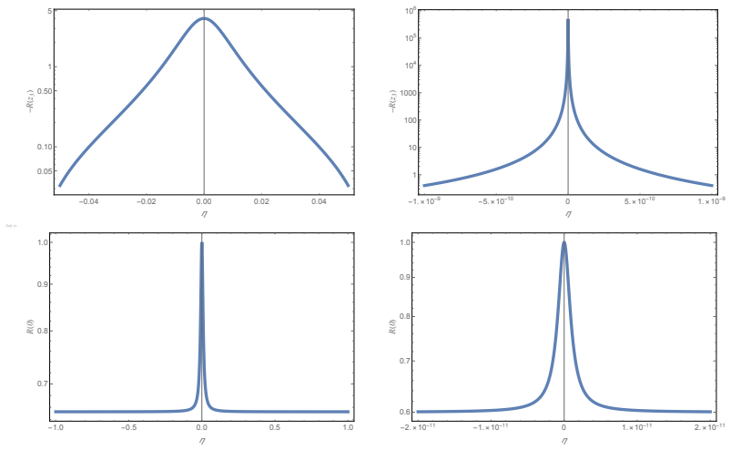
[Section 4.2, Example 3, and Section 4 conclusions] The stability analysis for the one-step MRE method covers the equal-magnitude case (Corollary 2) and shows that instability in individual components can be harmless when the corresponding η_i is small. Example 3, however, demonstrates that R(0) can be much smaller than 1, heavily damping slow modes, and that |R(z3)|>1 occurs for a whole neighborhood of η=0. The statement that the method is 'applicable in stiff case' is therefore only a partial conclusion; the paper should clearly state that a full stability guarantee for general initial data is not obtained, beyond what is admitted in Section 4.3 and the Conclusion.

minor comments (5)

[Throughout] There are several typos: 'experimantal', 'absoltely', 'Kramer' (for Cramer), 'withouth', 'whithout', and 'consequense'.
[Section 4.2, Example 3] The text says the graphs of −R(z3) are shown in 'the first row of Figure 3', but the illustration caption is 'Figure 2: Illustration of example 3.' The figure references should be corrected.
[Section 1, Eq. (2) and Section 4.1, Eq. (11)] The sign convention for α in the general method (α_j with a minus sign in Eq. (2)) and in the one-step method (α used positively in Eq. (11)) is confusing; the paper notes this, but a consistent notation would improve readability.
[Section 5.1] The phrase 'The computing of matrix W' and similar constructions are awkward; these sentences should be rephrased for clarity.
[Section 6.3] The text refers to 'Figure 6.3' in the discussion; this should be 'Figure 6' to match the figure caption.

Circularity Check

1 steps flagged · score 6.0 of 10

The theoretical order/zero-stability results are self-contained, but the heat-equation benchmark is constructed so the BDF solution lies in the MRMS subspace V, making the observed 'similar numerical solutions' a definitional identity rather than empirical evidence.

self definitional [Section 6.1, Eqs. (39)-(41); definition in Section 1, Eq. (9)]
"In order to exactly compute the error of our methods we construct a problem with preset solution of the form w_ij(t) = p(t)q_ij (40) by defining b(t) as b_ij(t) = p'(t)q_ij − p(t)/h^2(...). ... There is a simple but important observation: if y_BDF_k ∈ V and is unique, then y_k = y_BDF_k."

With this b(t), the discrete heat-equation RHS (39) reduces to f(t,w)=Aw+b=p(t)Lq+p'(t)q−p(t)Lq=p'(t)q, independent of w. Starting values are y_j=p(t_j)q, so every column of V in Eq. (8) is a scalar multiple of q; V=span{q}. The BDF equation then forces y_BDF_k to be a scalar multiple of q, hence y_BDF_k∈V. By the paper's own Eq. (9) plus the observation in Section 1, MRMS returns exactly y_BDF_k. Therefore the observed equality of BDF and MRMS errors (Section 6.4 and the abstract's 'both methods give similar numerical solutions') follows by construction from the test problem, not from any general subspace approximation property. The benchmark tests only reproduction of a known one-dimensional subspace, so it cannot validate the accuracy claim for general non-separable stiff problems.

full rationale

The core derivation of the paper is not circular. Theorem 1 proves order min{2k−1,p} by comparing the MRMS residual to the residual of a known explicit k-step method of order 2k−1 and using the BDF order condition; Lemma 1 proves zero-stability inheritance by showing that for f=0 the MRMS coefficients force the generating polynomial to be c_k^{-1} z^{k-p} ρ_BDF(z). Both arguments rely on standard external LMM facts, not on fitting the method's output. The linear stability analysis for the minimal residual Euler method is also self-contained, using minimax polynomial bounds on the diagonal model problem. The one genuine circular element is the numerical validation in Section 6. The benchmark is deliberately built from w_ij(t)=p(t)q_ij with b(t) chosen so the RHS is p'(t)q; consequently all vectors spanning V are multiples of q and the BDF solution lies in V, so MRMS equals BDF by definition. The paper's Section 6.4 claim that the errors are almost equal 'which means that ... y_BDF_k are well approximated by the elements of subspaces V' is therefore not evidence for the general unproved subspace approximation; it is forced by the construction. The paper honestly lists missing convergence proof as future work, so this is partial circularity in the experimental support rather than a circularity in the theoretical claims. Score 6 reflects one constructed prediction/validation that reduces by definition while the central order/zero-stability results remain externally grounded.

Assumptions & free parameters 0 free parameters · 4 assumptions · 0 invented entities

The central claims rest on standard LMM theory plus smoothness, invertibility, and rank assumptions. No data-fitted free parameters appear; the user-chosen k and p are method parameters, not fitted constants. No new physical or mathematical entity is postulated; MRMS is an algorithmic construction.

assumptions (4)

standard math There exists an explicit k-step linear multistep method of order 2k-1.
Invoked in the proof of Theorem 1 to provide a candidate vector Vγ with error O(τ^{2k}); this is a classical result in LMM theory.
domain assumption The BDF residual r is sufficiently smooth and locally invertible so that ||yk-y(tk)|| ≤ C||r(yk)-r(y(tk))|| via the mean-value theorem.
Theorem 1 proof relies on this inversion; for stiff systems with Jacobian eigenvalues near 1/τ this is not guaranteed, and no verification is provided.
domain assumption The thin least-squares problems are well-posed, i.e., the columns of W are linearly independent.
Proposition 2 characterizes well-posedness for the one-step case; the general method assumes the subspace V is non-degenerate so the coefficient vector is unique.
domain assumption Numerical experiments use exact starting values and a slowly-varying preset solution.
Section 6.1 takes starting values from the known exact solution (40)-(41), which removes startup error and favors the subspace approximation; the comparison does not test robust startup.

how reviews work

0 comments

Cite this review

Pith. "Pith review of Minimal residual multistep methods for large stiff non-autonomous linear problems." pith.science (2026). https://pith.science/paper/2SEJQF3A

@misc{pith2026190807984,
  author       = {Pith},
  title        = {Pith review of: Minimal residual multistep methods for large stiff non-autonomous linear problems},
  year         = {2026},
  howpublished = {\url{https://pith.science/paper/2SEJQF3A}},
  note         = {Machine review of arXiv:1908.07984}
}

abstract

The purpose of this work is to introduce a new idea of how to avoid the factorization of large matrices during the solution of stiff systems of ODEs. Starting from the general form of an explicit linear multistep method we suggest to adaptively choose its coefficients on each integration step in order to minimize the norm of the residual of an implicit BDF formula. Thereby we reduce the number of unknowns on each step from $n$ to $O(1)$, where $n$ is the dimension of the ODE system. We call this type of methods Minimal Residual Multistep (MRMS) methods. In the case of linear non-autonomous problem, besides the evaluations of the right-hand side of ODE, the resulting numerical scheme additionally requires one solution of a linear least-squares problem with a thin matrix per step. We show that the order of the method and its zero-stability properties coincide with those of the used underlying BDF formula. For the simplest analog of the implicit Euler method the properties of linear stability are investigated. Though the classical absolute stability analysis is not fully relevant to the MRMS methods, it is shown that this one-step method is applicable in stiff case. In the numerical experiment section we consider the fixed-step integration of a two-dimensional non-autonomous heat equation using the MRMS methods and their classical BDF counterparts. The starting values are taken from a preset slowly-varying exact solution. The comparison showed that both methods give similar numerical solutions, but in the case of large systems the MRMS methods are faster, and their advantage considerably increases with the growth of dimension. Python code with the experimantal code can be downloaded from the GitHub repository https://github.com/bfaleichik/mrms.

Figures

Figures reproduced from arXiv: 1908.07984 by the authors.

**Figure 2.** Illustration of example 3. Graphs of dependence of [PITH_FULL_IMAGE:figures/full_fig_p012_2.png] view at source ↗

**Figure 3.** Numerical results for example 3. Graphs of approximations to solution of the system [PITH_FULL_IMAGE:figures/full_fig_p013_3.png] view at source ↗

Figures from the paper (3 more)

**Figure 4.** Figure 4: The results of numerical experiment with stiff linear model problem (14) from [PITH_FULL_IMAGE:figures/full_fig_p015_4.png]

**Figure 5.** Figure 5: The results of numerical experiment with stiff linear model problem (14) from [PITH_FULL_IMAGE:figures/full_fig_p016_5.png]

**Figure 6.** Figure 6: The results of numerical experiment with the 2D heat equation (39). The dimension [PITH_FULL_IMAGE:figures/full_fig_p020_6.png]

Discussion (0). Continue with ORCID to comment.

Reference graph

Works this paper leans on

13 extracted references · 9 canonical work pages

[1]

P. J. Van Der Houwen, B. P. Sommeuer, A special class of multistep rungekutta methods with extended real stability interval, Ima Journal of 21 Numerical Analysis - IMA J NUMER ANAL 2 (1982) 183–209. doi: 10.1093/imanum/2.2.183

work page doi:10.1093/imanum/2.2.183 1982
[2]

Lebedev, Explicit diﬀerence schemes with variable time steps for solving stiﬀ systems of equations, in: L

V. Lebedev, Explicit diﬀerence schemes with variable time steps for solving stiﬀ systems of equations, in: L. Vulkov, J. Wasniewski, P. Yalamov (Eds.), Numerical Analysis and Its Applications, Vol. 1196 of Lecture Notes in Computer Science, Springer Berlin Heidelberg, 1997, pp. 274–283. doi: 10.1007/3-540-62598-4\_104 . URL http://dx.doi.org/10.1007/3-540...

doi:10.1007/3-540-62598-4 1997
[3]

Faleichik, I

B. Faleichik, I. Bondar, V. Byl, Generalized picard iterations: A class of iterated rungekutta methods for stiﬀ problems, Journal of Computational and Applied Mathematics 262 (2014) 37 – 50, selected Papers from NUMDIFF-13. doi:https://doi.org/10.1016/j.cam.2013.10.036. URL http://www.sciencedirect.com/science/article/pii/ S037704271300589X

work page doi:10.1016/j.cam.2013.10.036 2014
[4]

P. N. Brown, A. C. Hindmarsh, Matrix-free methods for stiﬀ systems of ode’s, SIAM J. Numer. Anal. 23 (3) (1986) 610–638. doi:10.1137/ 0723039. URL http://dx.doi.org/10.1137/0723039

doi:10.1137/0723039 1986
[5]

H. H. Rosenbrock, Some general implicit processes for the numerical solu- tion of diﬀerential equations, The Computer Journal 5 (4) (1963) 329–330. doi:10.1093/comjnl/5.4.329. URL https://dx.doi.org/10.1093/comjnl/5.4.329

doi:10.1093/comjnl/5.4.329 1963
[6]

Curtiss, J

C. Curtiss, J. O. Hirschfelder, Integration of stiﬀ equations, Proceedings of the National Academy of Sciences 38 (3) (1952) 235–243

work page 1952
[7]

J. M. Ortega, W. C. Rheinboldt, Iterative solution of nonlinear equations in several variables., Computer science and applied mathematics, Academic Press, 1970

work page 1970
[8]

Saad, Iterative Methods for Sparse Linear Systems, 2nd Edition, Society for Industrial and Applied Mathematics, Philadelphia, PA, USA, 2003

Y. Saad, Iterative Methods for Sparse Linear Systems, 2nd Edition, Society for Industrial and Applied Mathematics, Philadelphia, PA, USA, 2003

work page 2003

Show all 13 references

[9]

Hairer, G

E. Hairer, G. Wanner, Solving Ordinary Diﬀerential Equations II: Stiﬀ and Diﬀerential-Algebraic Problems, 2nd Edition, Springer-Verlag, New York, 1996

1996
[10]

J. W. Demmel, Applied Numerical Linear Algebra, SIAM, 1997. doi: 10.1137/1.9781611971446

1997 doi
[11]

Faleichik, Mrms methods experimental code, https://github.com/ bfaleichik/mrms (2019)

B. Faleichik, Mrms methods experimental code, https://github.com/ bfaleichik/mrms (2019)

2019
[12]

X. S. Li, M. Shao, A supernodal approach to incomplete lu factorization with partial pivoting, ACM Trans. Math. Softw. 37 (4) (2011) 43:1–43:20. doi:10.1145/1916461.1916467. URL http://doi.acm.org/10.1145/1916461.1916467 22

2011
[13]

Dahlquist, Convergence and stability in the numerical integration of ordinary diﬀerential equations, Mathematica Scandinavica 4 (1) (1956) 33– 53

G. Dahlquist, Convergence and stability in the numerical integration of ordinary diﬀerential equations, Mathematica Scandinavica 4 (1) (1956) 33– 53. URL http://www.jstor.org/stable/24490010 23

1956

Pith tools

Reviewed August 14, 2026 · model on record in the stance chip above.

[1] [1]

P. J. Van Der Houwen, B. P. Sommeuer, A special class of multistep rungekutta methods with extended real stability interval, Ima Journal of 21 Numerical Analysis - IMA J NUMER ANAL 2 (1982) 183–209. doi: 10.1093/imanum/2.2.183

work page doi:10.1093/imanum/2.2.183 1982

[2] [2]

Lebedev, Explicit diﬀerence schemes with variable time steps for solving stiﬀ systems of equations, in: L

V. Lebedev, Explicit diﬀerence schemes with variable time steps for solving stiﬀ systems of equations, in: L. Vulkov, J. Wasniewski, P. Yalamov (Eds.), Numerical Analysis and Its Applications, Vol. 1196 of Lecture Notes in Computer Science, Springer Berlin Heidelberg, 1997, pp. 274–283. doi: 10.1007/3-540-62598-4\_104 . URL http://dx.doi.org/10.1007/3-540...

doi:10.1007/3-540-62598-4 1997

[3] [3]

Faleichik, I

B. Faleichik, I. Bondar, V. Byl, Generalized picard iterations: A class of iterated rungekutta methods for stiﬀ problems, Journal of Computational and Applied Mathematics 262 (2014) 37 – 50, selected Papers from NUMDIFF-13. doi:https://doi.org/10.1016/j.cam.2013.10.036. URL http://www.sciencedirect.com/science/article/pii/ S037704271300589X

work page doi:10.1016/j.cam.2013.10.036 2014

[4] [4]

P. N. Brown, A. C. Hindmarsh, Matrix-free methods for stiﬀ systems of ode’s, SIAM J. Numer. Anal. 23 (3) (1986) 610–638. doi:10.1137/ 0723039. URL http://dx.doi.org/10.1137/0723039

doi:10.1137/0723039 1986

[5] [5]

H. H. Rosenbrock, Some general implicit processes for the numerical solu- tion of diﬀerential equations, The Computer Journal 5 (4) (1963) 329–330. doi:10.1093/comjnl/5.4.329. URL https://dx.doi.org/10.1093/comjnl/5.4.329

doi:10.1093/comjnl/5.4.329 1963

[6] [6]

Curtiss, J

C. Curtiss, J. O. Hirschfelder, Integration of stiﬀ equations, Proceedings of the National Academy of Sciences 38 (3) (1952) 235–243

work page 1952

[7] [7]

J. M. Ortega, W. C. Rheinboldt, Iterative solution of nonlinear equations in several variables., Computer science and applied mathematics, Academic Press, 1970

work page 1970

[8] [8]

Saad, Iterative Methods for Sparse Linear Systems, 2nd Edition, Society for Industrial and Applied Mathematics, Philadelphia, PA, USA, 2003

Y. Saad, Iterative Methods for Sparse Linear Systems, 2nd Edition, Society for Industrial and Applied Mathematics, Philadelphia, PA, USA, 2003

work page 2003