Statistical characterization of scattering delay in synthetic aperture radar imaging

Mikhail Gilman; Semyon Tsynkov

REVIEW 4 major objections 5 minor 27 references

Statistical characterization of scattering delay in synthetic aperture radar imaging

T0 review · 4 major / 5 minor · reviewed 2026-08-14 · deepseek-v4-flash

Challenge this review Re-run · record.json Download PDF Read on arXiv ↗ Review JSON

Pith's one-line read The paper claims that a two-threshold maximum-likelihood classifier, with thresholds set from speckle-simulation cumulative distributions and made contrast-independent by worst-case extremization, can keep delayed-versus-instantaneous SAR…

desk verdict Solid methodological paper: the confidence-level construction is correct and clearly presented, but the headline error-rate guarantee is proven only for the authors' simulation model, not for real SAR images. read the letter →

arxiv 1908.08124 v2 pith:IRE5T4WH submitted 2019-08-21 eess.IV

Mikhail Gilman , Semyon Tsynkov This is my paper · ORCID

classification eess.IV

keywords syntheticapertureradarcoordinate-delayimagingscatteringdelayrange-delayambiguityspecklestatisticsmaximumlikelihoodclassificationconfidencelevelstargetdiscrimination

verification ladder T0 review T1 audit T2 compute T3 formal

The pith

A machine-rendered reading of the paper's core claim, the machinery that carries it, and where it could break.

The reading

The paper tries to make the discrimination between instantaneous and delayed radar scatterers in coordinate-delay SAR images statistically reliable. It proposes a classifier with two thresholds on a log-likelihood score: above $l_+$ call the target delayed, below $l_-$ call it instantaneous, and in between declare uncertainty. The thresholds are quantiles of cumulative distribution functions built from simulated speckle ensembles; taking worst-case minima and maxima over target contrasts makes the thresholds contrast-independent. The payoff would be that a single SAR acquisition can carry a confidence label on the target type, which is currently missing because speckle makes deterministic discrimination unreliable.

What carries the argument

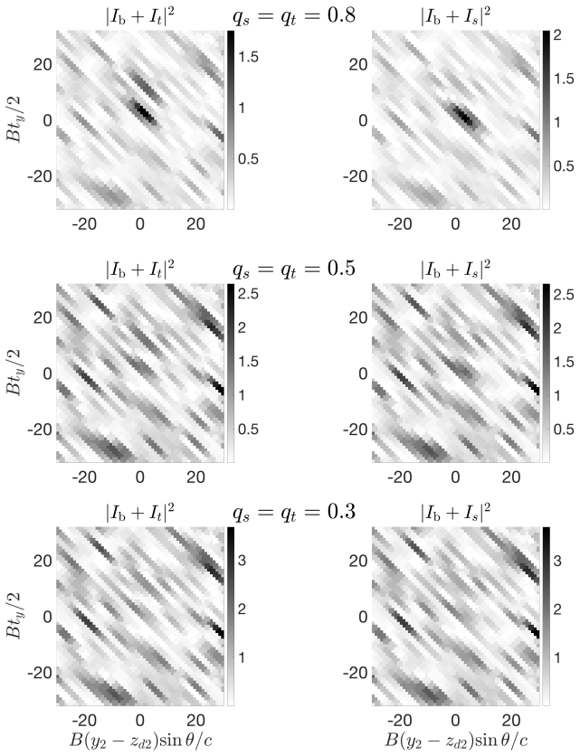
The load-bearing object is the coordinate-delay point spread function $W(t_y-t_z,\mathbf{y}-\mathbf{z})$, whose slow decay along the ambiguity lines $T_0=\mathrm{const}$ creates the range-delay ambiguity that makes instantaneous and delayed scatterers hard to separate. Around it, the paper places Gaussian white-noise models for the background, the delayed $t$-scatterer, and the instantaneous $s$-scatterer, from which the image second-order statistics (31)-(32) follow. Classification runs on the maximum-likelihood score $l=\log\hat{p}_t-\log\hat{p}_s$, and the confidence levels come from the cdf quantile equations (58), generalized to all contrasts by (61).

What would settle it

Run algorithm (52) with the contrast-independent thresholds from (61) on real coordinate-delay SAR images of a scene with independently calibrated instantaneous and delayed scatterers, and compare the decisions with ground truth; if the empirical misclassification rate exceeds $p$ for any target contrast, the bound does not transfer to practice.

Watch

Extended reading notes

Core claim

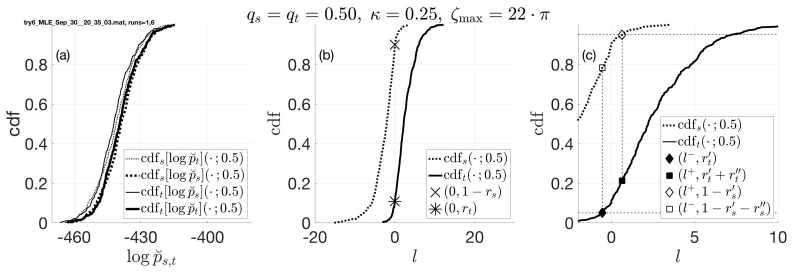
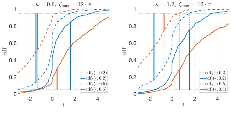
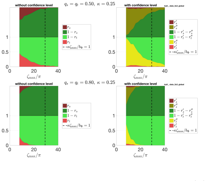
The paper's central claim is that a maximum-likelihood score $l=\log\hat{p}_t-\log\hat{p}_s$, the difference of the fitted likelihoods for the delayed and instantaneous models, can be turned into a calibrated three-outcome classifier. For known contrast, choosing $l_-$ and $l_+$ from $\mathrm{cdf}_t(l_-)=p$ and $\mathrm{cdf}_s(l_+)=1-p$ makes the misclassification rates exactly $p$. For unknown contrast, replacing these with the contrast-independent extremes of (61) yields $r'_s\le p$ and $r'_t\le p$ for every contrast distribution, and Monte Carlo simulations show the dependence of these rates on $\kappa$ and $\zeta_{\max}$.

Load-bearing premise

The error bound $p$ transfers to real radar images only if the Gaussian white-noise scattering models reproduce actual speckle statistics and the assumed independence between ambiguity lines holds; the paper never tests the thresholds against measured SAR data.

Editorial extensions

If this is right

A single SAR acquisition can be assigned a confidence label for 'delayed response present', because the thresholds need only system parameters and a simulation ensemble, not repeated imaging.
Operators can preset the maximum tolerable misclassification probability $p$ and get thresholds that keep $r'_s$ and $r'_t$ at or below $p$ for any unknown contrast distribution.
The required amount of delay is quantified: separation improves as $\zeta_{\max}$ grows, and the condition $\kappa\zeta_{\max}\gtrsim 20$ indicates when the ambiguity becomes resolvable.
Wider uncertainty intervals lower the error rates but raise the fraction of uncertain outcomes, an explicit trade-off measured by $r''_s$ and $r''_t$.
Saturation of reliable classification for $\kappa\gtrsim 0.4$ suggests a regime where increasing aperture width no longer improves discrimination quality.

Reading between the lines

Editorial extensions of the paper, not claims the author makes directly.

Extension: the same cdf-quantile construction could be reused for any binary SAR classification task whose two hypotheses have known covariance structure, not only delay detection.
Extension: the contrast-independent envelope of (61) is conservative for a known contrast distribution; averaging the cdfs over that distribution would shrink the uncertainty band while sacrificing the worst-case guarantee.
Extension: a calibrated delay-line corner reflector in a real SAR scene would provide a direct test of whether the simulated cdfs match reality; until then the $p$ bound is a property of the model world.
Extension: feeding the full eight-dimensional maximum-likelihood solution into a learned classifier is mentioned in the paper but not systematically explored; that parameter space remains an open testable extension.

Share X Bluesky LinkedIn Reddit HN

Signed reviews

No signed human review yet.

Editorial analysis

A structured set of objections, weighed in public.

Desk editor's note, referee report, and a circularity audit.

Desk Editor's Note

read the letter

Colleague,

You should know two things about this paper: the confidence-level construction is sound and clearly written, and the advertised error-rate guarantee is real only inside the simulation model. If you take the paper as a methods piece for coordinate-delay SAR, it is a legitimate advance over the authors' prior ML detector; if you take the headline as a statement about real radar images, there is no evidence yet.

What's new: the reject option in algorithm (52), the threshold selection via (58), and especially the contrast-independent version (61) that removes the need to know target contrast beforehand. That last bit is genuinely useful for automatic target recognition. The derivations in Sections 2-6 are internally coherent, the notation is heavy but the logic is traceable, and the figures honestly show that even moderate speckle makes classification hard. The paper does not hide its scaffolding: the abstract says 'simple statistical models', and the method is explicitly Monte-Carlo-based.

Where it is soft: the central guarantee is definitional. The thresholds are quantiles of the simulated cdfs, so r'_s and r'_t equal p by construction (eqs. 58-59). That is not a flaw in the algebra—it is exactly how confidence levels work—but it means the only load-bearing question is whether the Gaussian white-noise scattering model (23)-(29), the known delay profile (34), and the independence of ambiguity lines survive contact with real SAR speckle. The paper never tests that. Also, the contrast-independent min/max in (61) is computed over a finite q-grid (0.0 to 0.9, step 0.1), while the text says 'entire range'; that is a small overstatement. Section 6.2 assumes cdf continuity and monotonicity, which is standard but unverified. No code or data are shipped, which makes the Monte Carlo hard to reproduce.

None of this sinks the paper. The authors are honest about their scope, and within that scope the statistics are correct. But a revision should either add a real or measured SAR scene (or at least a convincing validation against measured speckle), or explicitly state that the p-bound applies to the model, not to any particular physical scene.

Recommendation: send it out. A serious referee can push on the model-to-reality transfer and the grid/monotonicity caveats, but the core methodological contribution deserves attention in the SAR imaging community.

Referee Report

4 major / 5 minor

Summary. This paper develops a statistical method for discriminating between instantaneous and delayed scatterers in coordinate-delay synthetic aperture radar (SAR) images. Building on the authors' prior work, the manuscript derives the point spread function and correlation structure of coordinate-delay images under circular Gaussian white-noise scattering models, formulates a maximum likelihood classifier based on the log-likelihood ratio l, and proposes to set classification thresholds l- and l+ as quantiles of simulated cumulative distribution functions. The authors claim that with these thresholds, the misclassification rates are kept at or below a preset level p for any probability distribution of target contrast when the thresholds are computed via the min/max procedure of Eq. (61). The paper includes Monte Carlo simulations showing the dependence of classification quality on parameters kappa and zeta_max.

Significance. The derivations in Sections 2-6 are internally coherent, and the paper provides a useful, explicit recipe for attaching confidence labels to SAR target classifications without knowing the target contrast. The point-spread function analysis and the closed-form correlation expressions are valuable and appear correct. The Monte Carlo experiments are described in sufficient detail to be reproduced, and the authors are explicit about the modeling assumptions. However, the headline error-rate guarantee is conditional on the stochastic scattering model (23)-(29) and the independence assumption of Section 4; these assumptions are not validated against measured SAR data or alternative generative models. As a result, the significance of the contribution rests on whether the model captures real speckle.

major comments (4)

[Section 6.2, Eqs. (58)-(59)] The error-rate guarantee is definitional. Equations (58) define l- and l+ as the p-quantile and (1-p)-quantile of the cdfs cdft and cdfs, and equations (59) then state that the misclassification rates r'_t and r'_s equal p. Consequently, the Monte Carlo results in Figures 5 and 6, which are produced from the same generators used to estimate those cdfs, demonstrate self-consistency rather than independent predictive performance. To support the advertised confidence levels, the method should be evaluated on data generated from a different statistical model (for example, with non-Gaussian clutter or correlated ambiguity lines) or on real coordinate-delay SAR images.
[Section 4 and Eq. (46b)] The key independence assumption is both built into the likelihood and enforced by the simulator. The text states that ambiguity lines spaced pi in zeta_d can be considered uncorrelated, and the product likelihood (46b) relies on this. The Figure 2 caption describes generating each ambiguity line independently, so the simulations cannot detect a failure of this assumption. The authors should provide a quantitative justification of the pi-spacing based on the correlation functions in Eqs. (31)-(32), or test sensitivity to correlated ambiguity lines.
[Section 6.3, Eq. (61)] The claim that error rates are bounded for any probability distribution of target contrasts is not fully supported. The minimum and maximum in Eq. (61) are evaluated on the finite grid q in {0.0, 0.1, ..., 0.9} with step 0.1, and no monotonicity of the quantiles with respect to q is demonstrated. If the worst-case contrast lies above 0.9, the computed thresholds will not satisfy cdft(l-;q) <= p and 1 - cdfs(l+;q) <= p for all q. Additionally, Section 6.2 assumes the cdfs are continuous and monotonic; this is not verified, and if the cdfs have flat regions or jumps, the quantile equations (58) may not have unique solutions.
[Section 7] No measured SAR data are used in the paper. All quantitative results are obtained from the synthetic ensemble generator based on the Gaussian white-noise models (23)-(29) and the known delay profile (34). As a consequence, the transfer of the p-guarantee to real radar imagery rests entirely on the unvalidated adequacy of these models. This limitation should be stated explicitly in the abstract and conclusion, and, ideally, a demonstration on a real or at least a strongly perturbed dataset should be included.

minor comments (5)

[Footnote 3] Footnote 3 uses the symbol 'xi_d' where 'zeta_d' is clearly intended; this should be corrected.
[Eq. (40)] Equation (40) writes the correlation as <I_mj,s-model I_mj',s-model> without a complex conjugate; to match Eq. (31), the second factor should be the conjugate, and the notation should be made consistent with the real-vector formalism in (42)-(44).
[Figures 3-6] The number of Monte Carlo realizations used to estimate the cdfs is not reported, and no error bars or confidence bands are given for the estimated quantiles l- and l+. This information would help the reader assess the statistical precision of the thresholds.
[Section 6.2] The term 'monotonic' is used without qualification; since cdfs are nondecreasing by definition, the authors should state whether they assume strict monotonicity, and in the flat-case they should note that the solutions to (58) may be non-unique.
[Figures 5 and 6] The captions describe the panels as 'flipped vertically' and refer to 'lower half' and 'upper half', which makes the presentation of the confusion-matrix entries difficult to follow; a clearer labeling scheme would improve readability.

Circularity Check

1 steps flagged · score 8.0 of 10

The p-guarantee is definitional: the thresholds are p-quantiles of the same simulated cdfs that define the claimed error rates.

self definitional [Section 6.2, equations (58)-(59)]
"Then, we define two values, l− and l+, implicitly as solutions to the following equations: cdft(l−;q) =p and cdfs(l+;q) = 1−p. (58) ... For an ensemble of datasets Q generated from the t-model, the frequency of the cases l(Q) < l− will be equal to p. ... r′t =P(l(Q)<l−| t-model)=p, (59a) ... r′s =P(l(Q) >l+| s-model)=p. (59b)"

Equation (58) defines l− and l+ as the p-th and (1−p)-th quantiles of the very cdfs that, via (54)-(55), are the probabilities appearing in (59). The equalities r′t=p and r′s=p are therefore not an independent finding or a prediction; they are a restatement of the quantile definition. These cdfs are built from Monte Carlo ensembles generated from the paper's own Gaussian white-noise scattering models (23)-(29) and (37), so the advertised error bound is enforced by construction on the simulation generator. The only content that could falsify the guarantee—agreement of these cdfs with real coordinate-delay SAR imagery—is not tested; Figures 5-6 evaluate the same simulated ensembles used for calibration.

full rationale

The formal derivation from (58) to (59) is valid, but it is tautological: the thresholds are chosen as quantiles of the cdfs, and the claimed error rates are exactly those quantiles. The contrast-independent extension (61) is a legitimate pointwise min/max bound conditional on the cdfs, but it does not repair the model-dependence of the cdfs themselves. The paper's Section 4 'simplified treatment' assumes data on different ambiguity lines are uncorrelated, and the Figure 2 simulator generates each ambiguity line independently 'according to (31)', so the Monte Carlo experiments cannot validate that independence; they hard-code it. Similarly, the Gaussianity and the known delay profile (34) are built into the generator. Section 6.3's implementation of (61) on the q-grid {0.0,...,0.9} with step 0.1 is a generalization gap relative to the claim of 'any probability distributions of contrasts q', though this is a limitation rather than a circular step. The self-citations to [7] supply the imaging kernel, the ML likelihood framework, and the Monte Carlo procedure; they are prior work by the same authors but are not used as a uniqueness theorem, so they are not the main circularity. The central circularity is that the headline p-bound is a definitional, in-sample statement: thresholds calibrated on simulated cdfs are 'validated' by the same cdfs and the same simulator. Score 8 reflects that the central claim reduces by construction to its own definitions, with no external benchmark or measured SAR data to test the model transfer.

Assumptions & free parameters 5 free parameters · 6 assumptions · 0 invented entities

The central claim rests on a chain of modeling assumptions inherited from [6,7], on a finite contrast grid, and on Monte Carlo cdfs derived from the same statistical models used to define the likelihood. No new physical entity is introduced; the only invented objects are statistical target models that the paper itself acknowledges as simplifications. The key unstated cost is that confidence thresholds are calibrated on simulated data and inherit every modeling error without an external check.

free parameters (5)

Contrast grid for equation (61) = q = 0.0, 0.1, ..., 0.9
Used to replace the min and max over all target contrasts in (61) by a finite computation; contrasts above 0.9 and between grid points are not covered by the guarantee.
Noise contrast pn = 0.1
Fixed in all simulations at the end of Section 4 because its effect was considered not prominent; this choice affects the simulated image statistics.
Minimum delay cutoff zeta_min = 3*pi
Introduced in Section 5 to cut off transitional effects near zeta = 0; it selects which ambiguity lines enter the classification and therefore affects the thresholds.
Sampling points per ambiguity line Nm and locations psi = Nm=2, psi_m1=zeta_d, psi_m2=-zeta_d
Chosen in a footnote in Section 6.2 to maximize the expected intensity of at least one inhomogeneous image component; the confidence thresholds depend on this sampling design.
Scenario parameters kappa and zeta_max = kappa = 2.5, zeta_max = 5*pi for Figure 2; varied in Figures 5 and 6
These are simulation scenario parameters rather than fitted quantities, but the reported error rates and conclusions are conditional on the chosen ranges.

assumptions (6)

domain assumption Circular Gaussian white-noise models for background, t-scatterer, and s-scatterer in equations (23)-(29)
These stochastic models are adopted from prior work [6,7] and are not validated against measured SAR data in this paper; all simulated ensembles inherit them.
domain assumption Ambiguity lines spaced by pi are statistically uncorrelated
Invoked in Section 4 to factor the likelihood as a product over m in equation (46b); it is an approximation whose accuracy is not quantified.
domain assumption The cumulative distribution functions of l are continuous and monotonic
Assumed in Section 6.2 so that equation (58) has unique solutions l- and l+; real finite-sample cdfs are step functions and may be locally nonmonotone.
ad hoc to paper Finite grid q in [0,0.9] spans the entire range of target contrasts
Section 6.3 computes the worst-case thresholds over this grid only; the paper gives no argument that contrasts outside the grid cannot violate the claimed error bound.
domain assumption Speckle in real SAR follows the circular Gaussian statistics of equation (25)
The paper cites [6,9] for speckle theory, but no experimental verification is provided here, and all subsequent simulation results depend on this assumption.
standard math Standard SAR approximations: start-stop, angular coherence, small aperture angle, chirp assumptions
Used to derive the coordinate-delay imaging operator in equations (5)-(10); these are standard in the SAR literature and are not the focus of the paper.

how reviews work

0 comments

Cite this review

Pith. "Pith review of Statistical characterization of scattering delay in synthetic aperture radar imaging." pith.science (2026). https://pith.science/paper/IRE5T4WH

@misc{pith2026190808124,
  author       = {Pith},
  title        = {Pith review of: Statistical characterization of scattering delay in synthetic aperture radar imaging},
  year         = {2026},
  howpublished = {\url{https://pith.science/paper/IRE5T4WH}},
  note         = {Machine review of arXiv:1908.08124}
}

read the original abstract

Distinguishing between the instantaneous and delayed scatterers in synthetic aperture radar (SAR) images is important for target identification and characterization. To perform this task, one can use the autocorrelation analysis of coordinate-delay images. However, due to the range-delay ambiguity the difference in the correlation properties between the instantaneous and delayed targets may be small. Moreover, the reliability of discrimination is affected by speckle, which is ubiquitous in SAR images, and requires statistical treatment. Previously, we have developed a maximum likelihood based approach for discriminating between the instantaneous and delayed targets in SAR images. To test it, we employed simple statistical models. They allowed us to simulate ensembles of images that depend on various parameters, including aperture width and target contrast. In the current paper, we enhance our previously developed methodology by establishing confidence levels for the discrimination between the instantaneous and delayed scatterers. Our procedure takes into account the difference in thresholds for different target contrasts without making any assumptions about the statistics of those contrasts.

Figures

Figures reproduced from arXiv: 1908.08124 by the authors.

**Figure 1.** Plots of h|It | 2 i and h|Is| 2 i for different values of ζmax and κ, see (34) and (22). The dashed lines passing through the origin indicate the ambiguity direction, see (11),(13). For the middle row of plots, the condition κζmax & 20 (see (35)) is satisfied, and the difference in the orientation of the parallelogramshaped level lines is more apparent than for the top and bottom rows. 12 [PITH_FULL_IMAGE:figures/… view at source ↗

**Figure 2.** Simulated coordinate-delay SAR images with different contrasts. [PITH_FULL_IMAGE:figures/full_fig_p015_2.png] view at source ↗

**Figure 3.** Cumulative distribution functions (cdf) for ensembles generated [PITH_FULL_IMAGE:figures/full_fig_p021_3.png] view at source ↗

Figures from the paper (3 more)

**Figure 4.** Figure 4: Separation between the graphs of cdfs(· ; q) and cdft(· ; q) for different values of κ and q. The thick colored vertical bars indicate the percentage of uncertain classifications for the ensembles generated from the s-model (the left set of bars in each plot) and t-mo…

**Figure 5.** Figure 5: Dependence of the discrimination quality on [PITH_FULL_IMAGE:figures/full_fig_p026_5.png]

**Figure 6.** Figure 6: Dependence of discrimination quality on κ, see (22). The notations are the same as in [PITH_FULL_IMAGE:figures/full_fig_p027_6.png]

Discussion (0). Continue with ORCID to comment.

Reference graph

Works this paper leans on

27 extracted references · 27 canonical work pages

[1]

A. S. Monin and A. M. Yaglom. Statistical Fluid Mechanics: Mechanics of Turbulence. Volume 1. The MIT Press, Cambridge, MA, 1971. 2

work page 1971
[2]

S. M. Rytov, Yu. A. Kravtsov, and V. I. Tatarskii. Principles of Statisti- cal Radiophysics. Volume 4. Wave Propagation Through Random Media . Springer-Verlag, Berlin, 1989. Translated from the second Russian edition by Alexander P. Repyev. 2

work page 1989
[3]

The inﬂuence of equatorial scintillation on L- band SAR image quality and phase

Franz J Meyer, Kancham Chotoo, Susan D Chotoo, Barton D Huxtable, and Charles S Carrano. The inﬂuence of equatorial scintillation on L- band SAR image quality and phase. IEEE Transactions on Geoscience and Remote Sensing , 54(2):869–880, 2016. 2

work page 2016
[4]

A multiscale approach to synthetic aperture radar in dispersive random media

Josselin Garnier and Knut Sølna. A multiscale approach to synthetic aperture radar in dispersive random media. Inverse Problems, 29:054006 (18pp), 2013. 2 28

work page 2013
[5]

Gilman and S

M. Gilman and S. Tsynkov. Mathematical analysis of SAR imaging through a turbulent ionosphere. In Michail D. Todorov, editor, Applica- tion of Mathematics in Technical and Natural Sciences: 8th International Conference for Promoting the Application of Mathematics in Technical and Natural Sciences — AMiTaNS’17 , volume 1895 of AIP Conference Proceedings, p...

work page
[6]

Understanding Synthetic Aperture Radar Images

Chris Oliver and Shaun Quegan. Understanding Synthetic Aperture Radar Images. Artech House Remote Sensing Library. Artech House, Boston,

work page
[7]

Detection of delayed target re- sponse in SAR

Mikhail Gilman and Semyon Tsynkov. Detection of delayed target re- sponse in SAR. Inverse Problems, 35(8):085005, July 2019. 2, 3, 6, 8, 11, 18, 19, 20, 25, 26

work page 2019
[8]

Hyperspectral SAR

Matthew Ferrara, Andrew Homan, and Margaret Cheney. Hyperspectral SAR. IEEE Transactions on Geoscience and Remote Sensing, 55(3):1–14, March 2017. 2, 3

work page 2017

Show all 27 references

[9]

Statistical properties of laser speckle patterns

Joseph W Goodman. Statistical properties of laser speckle patterns. In Laser speckle and related phenomena , pages 9–75. Springer, 1984. 2, 8, 9

1984
[10]

Transionospheric synthetic aperture imaging

Mikhail Gilman, Erick Smith, and Semyon Tsynkov. Transionospheric synthetic aperture imaging . Applied and Numerical Harmonic Analysis. Birkh¨ auser/Springer, Cham, Switzerland, 2017. 4

2017
[11]

http://dlmf.nist.gov/, Release 1.0.23 of 2019-06-15

NIST Digital Library of Mathematical Functions . http://dlmf.nist.gov/, Release 1.0.23 of 2019-06-15. F. W. J. Olver, A. B. Olde Daalhuis, D. W. Lozier, B. I. Schneider, R. F. Boisvert, C. W. Clark, B. R. Miller and B. V. Saunders, eds. 7

2019
[12]

Handbook of radar scattering statistics for terrain (Artech House Remote Sensing Library)

Fawwaz T Ulaby and M Craig Dobson. Handbook of radar scattering statistics for terrain (Artech House Remote Sensing Library) . Artech House, Norwood, MA, USA, 1989. 9

1989
[13]

Allen and Stephen L

Jeﬀery C. Allen and Stephen L. Hobbs. Spectral estimation of non- stationary white noise. J. Franklin Inst. B , 334(1):99–116, 1997. 9

1997
[14]

A computational approach to edge detection

John Canny. A computational approach to edge detection. IEEE Trans- actions on pattern analysis and machine intelligence, PAMI-8(6):679–698,
[15]

Gaussian-based edge-detection methods—a survey

Mitra Basu. Gaussian-based edge-detection methods—a survey. IEEE Transactions on Systems, Man, and Cybernetics, Part C (Applications and Reviews), 32(3):252–260, 2002. 11, 14

2002
[16]

Edge detection techniques—an overview

Djemel Ziou, Salvatore Tabbone, et al. Edge detection techniques—an overview. Pattern Recognition and Image Analysis C/C of Raspozna- vaniye Obrazov I Analiz Izobrazhenii , 8:537–559, 1998. 11, 14

1998
[17]

Theory of edge detection

David Marr and Ellen Hildreth. Theory of edge detection. Proc. R. Soc. Lond. B, 207(1167):187–217, 1980. 11, 14

1980
[18]

Scheaﬀer

William Mendenhall and Richard L. Scheaﬀer. Mathematical statistics with applications. Duxbury Press, North Scituate, Mass., 1973. 16, 17, 20

1973
[19]

Dispersive scattering for radar-based target classiﬁcation and duct-induced image artifact mitigation

Brett Borden. Dispersive scattering for radar-based target classiﬁcation and duct-induced image artifact mitigation. In NATO Symposium on Non-Cooperative Air Target Identﬁcation Using Radar , pages 14.1–14.7. North Atlantic Treaty Organization, Research and Technology Organiza...

1998
[20]

Chen and Hao Ling

Victor C. Chen and Hao Ling. Time-frequency transforms for radar imag- ing and signal analysis . Artech House Radar Library. Artech House, Nor- wood, MA, 2002. 26

2002
[21]

Christopher M. Bishop. Pattern recognition and machine learning. Infor- mation Science and Statistics. Springer, New York, 2006. 27

2006
[22]

Imagenet classi- ﬁcation with deep convolutional neural networks

Alex Krizhevsky, Ilya Sutskever, and Geoﬀrey E Hinton. Imagenet classi- ﬁcation with deep convolutional neural networks. In Advances in neural information processing systems, pages 1097–1105, 2012. 27

2012
[23]

Systematic evalua- tion of convolution neural network advances on the Imagenet

Dmytro Mishkin, Nikolay Sergievskiy, and Jiri Matas. Systematic evalua- tion of convolution neural network advances on the Imagenet. Computer Vision and Image Understanding , 161:11 – 19, 2017. 27

2017
[24]

Deep learning in remote sensing: a comprehensive review and list of resources

Xiao Xiang Zhu, Devis Tuia, Lichao Mou, Gui-Song Xia, Liangpei Zhang, Feng Xu, and Friedrich Fraundorfer. Deep learning in remote sensing: a comprehensive review and list of resources. IEEE Geoscience and Remote Sensing Magazine, 5(4):8–36, 2017. 28

2017
[25]

SAR target recognition based on deep learning

Sizhe Chen and Haipeng Wang. SAR target recognition based on deep learning. In Data Science and Advanced Analytics (DSAA), 2014 Inter- national Conference on, pages 541–547. IEEE, 2014. 28 30

2014
[26]

A deep learning approach to the synthetic and measured paired and labeled experiment (SAMPLE) challenge problem

Theresa Scarnati and Benjamin Lewis. A deep learning approach to the synthetic and measured paired and labeled experiment (SAMPLE) challenge problem. In Algorithms for Synthetic Aperture Radar Imagery XXVI, volume 10987, page 109870G. International Society for Optics and Photo...

2019
[27]

The elements of statistical learning

Trevor Hastie, Robert Tibshirani, and Jerome Friedman. The elements of statistical learning . Springer Series in Statistics. Springer, New York, second edition, 2009. Data mining, inference, and prediction. 28 31

2009

Pith tools

Reviewed August 14, 2026 · model on record in the stance chip above.

[1] [1]

A. S. Monin and A. M. Yaglom. Statistical Fluid Mechanics: Mechanics of Turbulence. Volume 1. The MIT Press, Cambridge, MA, 1971. 2

work page 1971

[2] [2]

S. M. Rytov, Yu. A. Kravtsov, and V. I. Tatarskii. Principles of Statisti- cal Radiophysics. Volume 4. Wave Propagation Through Random Media . Springer-Verlag, Berlin, 1989. Translated from the second Russian edition by Alexander P. Repyev. 2

work page 1989

[3] [3]

The inﬂuence of equatorial scintillation on L- band SAR image quality and phase

Franz J Meyer, Kancham Chotoo, Susan D Chotoo, Barton D Huxtable, and Charles S Carrano. The inﬂuence of equatorial scintillation on L- band SAR image quality and phase. IEEE Transactions on Geoscience and Remote Sensing , 54(2):869–880, 2016. 2

work page 2016

[4] [4]

A multiscale approach to synthetic aperture radar in dispersive random media

Josselin Garnier and Knut Sølna. A multiscale approach to synthetic aperture radar in dispersive random media. Inverse Problems, 29:054006 (18pp), 2013. 2 28

work page 2013

[5] [5]

Gilman and S

M. Gilman and S. Tsynkov. Mathematical analysis of SAR imaging through a turbulent ionosphere. In Michail D. Todorov, editor, Applica- tion of Mathematics in Technical and Natural Sciences: 8th International Conference for Promoting the Application of Mathematics in Technical and Natural Sciences — AMiTaNS’17 , volume 1895 of AIP Conference Proceedings, p...

work page

[6] [6]

Understanding Synthetic Aperture Radar Images

Chris Oliver and Shaun Quegan. Understanding Synthetic Aperture Radar Images. Artech House Remote Sensing Library. Artech House, Boston,

work page

[7] [7]

Detection of delayed target re- sponse in SAR

Mikhail Gilman and Semyon Tsynkov. Detection of delayed target re- sponse in SAR. Inverse Problems, 35(8):085005, July 2019. 2, 3, 6, 8, 11, 18, 19, 20, 25, 26

work page 2019

[8] [8]

Hyperspectral SAR

Matthew Ferrara, Andrew Homan, and Margaret Cheney. Hyperspectral SAR. IEEE Transactions on Geoscience and Remote Sensing, 55(3):1–14, March 2017. 2, 3

work page 2017