REVIEW 2 major objections 4 minor 43 references
Regression Analysis of Unmeasured Confounding
T0 review · 2 major / 4 minor · reviewed 2026-08-14 · deepseek-v4-flash
Pith's one-line read A confounding interval for an adjusted regression slope can be computed exactly by checking at most 88 candidate parameter tuples, so unmeasured confounding becomes quantifiable rather than a caveat.
desk verdict Good idea with a clean implementation, but the central exactness proof has an algebraic error in the Lagrange step and the finite-set enumeration is not yet justified. read the letter →
The pith
A machine-rendered reading of the paper's core claim, the machinery that carries it, and where it could break.
The reading
What carries the argument
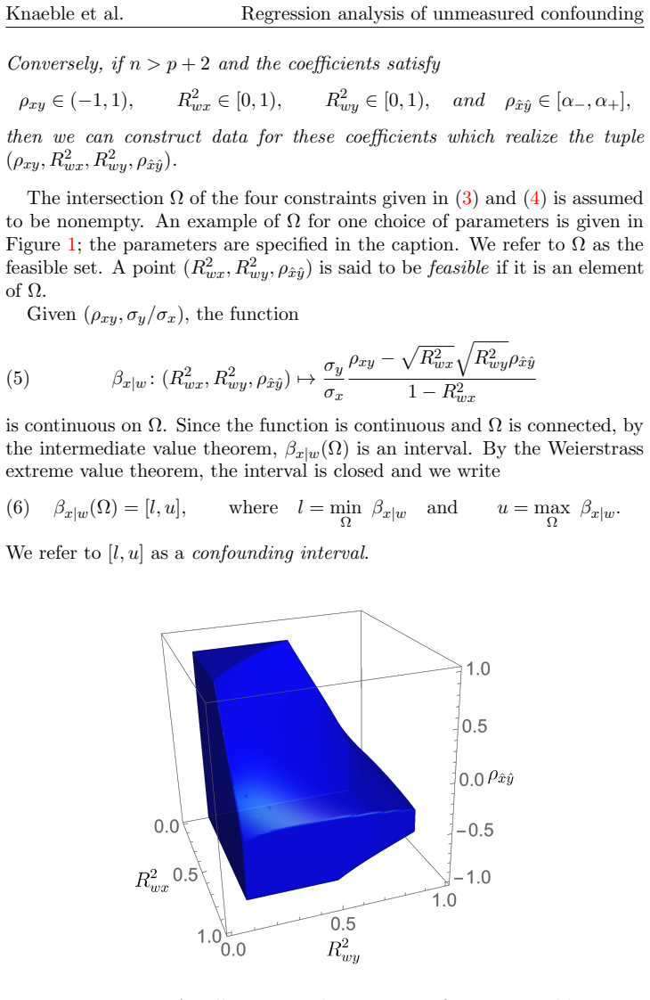
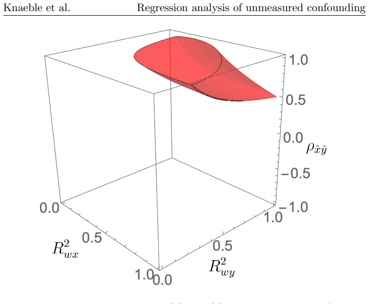
The load-bearing object is the rational map $\beta_{x|w}$ defined by equation (2), together with the feasible set $\Omega$ carved out by three box constraints and the realizability interval (4). The mechanism that carries the argument is constraint enumeration: because $\beta_{x|w}$ is monotone in $\rho_{\hat{x}\hat{y}}$ and in the confounding-strength coordinates except in special cases, an optimum must occur with at least two constraints active, and enumerating the combinations of active bounds, solving quadratics where needed and applying the Lagrange condition where the realizability curve is active, produces at most 88 candidate points. This turns a nonconvex continuous optimization problem into finite enumeration.
What would settle it
Run a numerical search: for fixed $\rho_{xy}$ and $\sigma_y/\sigma_x$, generate many random feasible tuples on dense grids inside $\Omega$ for several bound sets, evaluate $\beta_{x|w}$, and compare the extremes against the 88-point enumeration; any sampled value outside $[l,u]$ would disprove Proposition 2.2. To test the bounds' validity rather than the enumeration, simulate data with known unmeasured $w$, compute the true $\beta_{x|w}$, and construct bounds that exclude the true tuple; the method will then return an interval missing the true value, confirming that the diagnostic power comes from the bounds.
Extended reading notes
Core claim
The paper's central claim is Proposition 2.2: for any nonempty feasible set $\Omega$ defined by box constraints on $(R^2_{wx}, R^2_{wy}, \rho_{\hat{x}\hat{y}})$ together with the realizability constraint (4), the minimum and maximum of the adjusted slope $\beta_{x|w}$ over $\Omega$ are attained on a finite subset $S$ with $|S| \le 88$. Therefore the confounding interval $[l,u] = \beta_{x|w}(\Omega)$ can be computed exactly by evaluating $\beta_{x|w}$ at the candidate points in $S$. The candidates are generated by solving the stationarity conditions that arise when subsets of the eight inequality constraints are active, including quadratic formulas and Lagrange multiplier conditions; points where no constraints are active cannot be optimal because the objective is monotone in at least one free coordinate. The formula being propagated is $\beta_{x|w} = \frac{\sigma_y}{\sigma_x}\frac{\rho_{xy} - R_{wx}R_{wy}\rho_{\hat{x}\hat{y}}}{1-R^2_{wx}}$, and the realizability constraint ensures that every tuple considered can actually arise from real data.
Load-bearing premise
The entire calculation inherits the researcher's bounds on the three confounding statistics, and the feasibility formula silently assumes the product of the two confounding strengths is positive, so a zero lower bound (as in the worked example) needs a limiting interpretation not supplied in the text.
Editorial extensions
If this is right
- For any user-specified bounds that make the feasible set nonempty, the algorithm returns the exact endpoints of the confounding interval rather than a Monte Carlo or grid approximation.
- The interval $[l,u]$ is the full set of adjusted slopes compatible with the bounds: a true slope outside it implies that at least one stated bound was wrong.
- Researchers can report a confounding interval alongside the usual confidence interval, separating sampling uncertainty from uncertainty about unmeasured attributes.
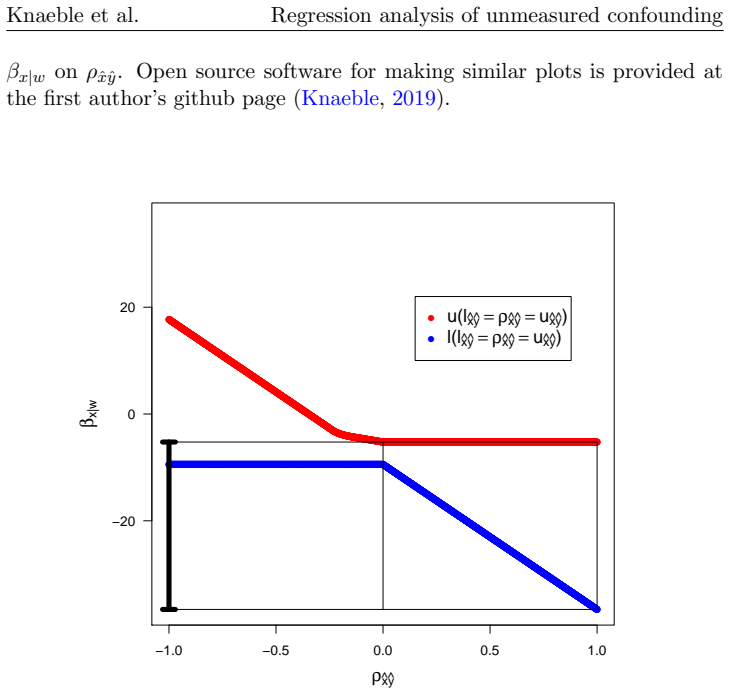
- Tighter subject-matter bounds on the correlation between fitted treatment and fitted outcome can directly shrink the interval, as the diet example shows.
- Because the number of candidate points is bounded by 88 independent of the number of unmeasured confounders, the computation stays trivial as the confounding set grows.
Reading between the lines
- Not in the paper: the same finite-candidate machinery applies to any function of $(R^2_{wx}, R^2_{wy}, \rho_{\hat{x}\hat{y}})$ that is monotone in at least one coordinate on $\Omega$, such as the partial correlation in equation (9), so the enumeration could be reused for other sensitivity targets.
- Not in the paper: if the bounds are estimated from measured subsets of $w$ rather than being subject-matter certainties, a natural next step is to propagate sampling error in the bounds into a conservative widening of the interval, perhaps by bootstrapping the bound estimates.
- Not in the paper: the realizability constraint in (4) divides by $R_{wx}R_{wy}$, so the case where a lower bound is zero, as in the worked example's $l^2_y = 0$, requires a limiting argument that the text does not supply.
Signed reviews
Editorial analysis
A structured set of objections, weighed in public.
Referee Report
Summary. The manuscript introduces a 'confounding interval' for the adjusted slope βx|w in linear regression with unmeasured confounders. It uses three parameters—R²wx, R²wy, and the correlation ρhat between fitted values—and propagates user-specified bounds through an algebraic identity (Proposition 1.1) and a realizability condition (Proposition 2.1). The main algorithmic claim (Proposition 2.2) is that the endpoints of the interval are attained on a finite set S of at most 88 candidate triples, so exact enumeration is possible. A case study on PBDE exposure and IQ illustrates the method.
Significance. If Proposition 2.2 were correct, the paper would provide a useful, computationally exact sensitivity analysis with interpretable confounding parameters, and it would improve on earlier sign-reversal conditions. The identity in Proposition 1.1 is cleanly proved with projections, and the paper ships Python and R implementations. However, the proof of the central enumeration contains a load-bearing algebraic error, and the method as stated mishandles the zero lower-bound cases used in the application. The contribution therefore needs substantial correction before its claims can be relied upon.
major comments (2)
- [Appendix C / Proposition 2.2] The Lagrange-multiplier step for the case where (3c) and (4) are active is not correct. With g(Rwx,Rwy)=b_rho RwxRwy ± sqrt(1−Rwx²)sqrt(1−Rwy²), the printed derivative contains a spurious factor of 2 and a spurious (1+Rwy²)^{1/2}; the correct derivative is ∂g/∂Rwx = b_rho Rwy ∓ Rwx sqrt(1−Rwy²)/sqrt(1−Rwx²), and similarly for ∂g/∂Rwy. The printed ratio therefore does not imply Rwx=Rwy, and the candidates (7b) and (7c) are not the only stationary points on this surface. A concrete check: take ρxy=0.85, σy/σx=1, l²x=l²y=0.1, u²x=u²y=0.9, and l_rhohat=u_rhohat=0.8. The point (R²wx,R²wy,ρhat)≈(0.659,0.326,0.8) satisfies the correct Lagrange equations and (4), is feasible, and is not any of the forms (7a)–(7g); its βx|w is about 1.406, while the feasible candidates of the listed forms include (0.5,0.1,0.8) with value about 1.342. Thus the stated enumeration can return an interval that is too narrow, contradicting equation (6).
- [Section 2, constraints (3a)–(3c) and (4)] The feasibility condition (4) divides by RwxRwy, so it is undefined when R²wx=0 or R²wy=0. The main text nevertheless allows l²x=0 and l²y=0 in (3a) and (3b), and the Section 3 example sets l²y=0 and reports [−36.60,17.71]. Proposition 2.1's converse also nominally covers R²wx=0 or R²wy=0. The paper must either require 0<l²x and 0<l²y, or treat the zero cases separately, for example by a limiting argument or by a different parametrization of (4). As written, the example's interval is not supported by the stated theory.
minor comments (4)
- [Appendix C and Proposition 2.2, line (7g)] The formula in (7g) appears to contain a typo: for the case (3b)+(3c)+(4), the quadratic should be written in terms of b²y, not b²x, in the argument of q²±; as printed, the formula does not match the derivation that precedes it.
- [Proposition 2.2, line (7e)] There is a notation inconsistency in (7e): S is a set of triples (R²wx,R²wy,ρhat), so the first two entries should be the squared bounds b²x and b²y, but the formula writes bx and by without squares.
- [Figure 2 caption] The caption reports u²y=50%, whereas the text of Section 3 specifies 0≤R²wy≤0.2; one of these is a typo and should be corrected.
- [Appendix C] The word 'Propositon' appears instead of 'Proposition'; this is a minor typo but should be fixed.
Circularity Check
No significant circularity: the methodology propagates user-specified bounds through an independently derived algebraic identity, and the central optimization result is proven in-appendix rather than assumed from prior work.
full rationale
The paper's central claim is Proposition 2.2, an optimization theorem stating that extrema of the adjusted slope over the feasible set are attained on a finite set. This claim does not reduce to its inputs: the objective in equation (5) comes from Proposition 1.1, which is proved in Appendix A from projection matrices and the partial-correlation identity (8), not assumed or fitted. The realizability constraint (4) in Proposition 2.1 is likewise derived from the same identity together with the fact that a partial correlation lies in [-1,1], and a converse construction is sketched; it is not imposed as a paper-specific ansatz. The inputs of the method are analyst-specified bounds on three confounding parameters, and the output interval in equation (6) is definitionally the range of the adjusted slope under those constraints. This is propagation of a stated assumption through a derived equation, not fitting a parameter to data and then relabeling it as a prediction. The self-citations to Knaeble and Dutter (2017) for equation (2) and to other prior work are not load-bearing: an alternative proof is included in Appendix A, and no uniqueness claim or substantive assumption is imported solely from the authors' own papers. The possible algebraic error in the Lagrange-multiplier step of Appendix C is a correctness risk but not circularity, since an incorrect derivative computation does not make the conclusion equivalent to the inputs. The worked example explicitly labels its bounds as illustrative, so there is no hidden fitting of the target interval. Overall, no step in the derivation chain equates the output to the input by construction.
Assumptions & free parameters
free parameters (3)
- lower and upper bounds on R2wx =
l2x = 0.1, u2x = 0.5 in example
- lower and upper bounds on R2wy =
l2y = 0.0, u2y = 0.2 in example
- lower and upper bounds on ρ_hatx_haty =
l_hatx_haty = -1, u_hatx_haty = 1 (default), then 0 to 1 in refined example
assumptions (4)
- domain assumption The true data-generating process is the linear model y = β0|w + βx|w x + β1 w1 + ... + βp wp + ε with least-squares-consistent errors.
- domain assumption The unmeasured confounding set w is admissible for causal interpretation, i.e., potential outcomes are independent of treatment conditional on w.
- domain assumption The user-specified bounds (3a-c) contain the true values of R2wx, R2wy, and ρ_hatx_haty for the unmeasured w.
- ad hoc to paper RwxRwy > 0, so that the feasibility constraint (4) is defined.
Cite this review
Pith. "Pith review of Regression Analysis of Unmeasured Confounding." pith.science (2026). https://pith.science/paper/OBXV5OZJ
@misc{pith2026190808596,
  author       = {Pith},
  title        = {Pith review of: Regression Analysis of Unmeasured Confounding},
  year         = {2026},
  howpublished = {\url{https://pith.science/paper/OBXV5OZJ}},
  note         = {Machine review of arXiv:1908.08596}
}
abstract
When studying the causal effect of $x$ on $y$, researchers may conduct regression and report a confidence interval for the slope coefficient $\beta_{x}$. This common confidence interval provides an assessment of uncertainty from sampling error, but it does not assess uncertainty from confounding. An intervention on $x$ may produce a response in $y$ that is unexpected, and our misinterpretation of the slope happens when there are confounding factors $w$. When $w$ are measured we may conduct multiple regression, but when $w$ are unmeasured it is common practice to include a precautionary statement when reporting the confidence interval, warning against unwarranted causal interpretation. If the goal is robust causal interpretation then we can do something more informative. Uncertainty in the specification of three confounding parameters can be propagated through an equation to produce a confounding interval. Here we develop supporting mathematical theory and describe an example application. Our proposed methodology applies well to studies of a continuous response or rare outcome. It is a general method for quantifying error from model uncertainty. Whereas confidence intervals are used to assess uncertainty from unmeasured individuals, confounding intervals can be used to assess uncertainty from unmeasured attributes.
Figures
Reference graph
Works this paper leans on
-
[1]
Angrist, J. and Pischke, J. (2009). Mostly Harmless Economics: An Empericist’s Companion. Princeton University Press
work page 2009
-
[2]
Public Health Statement on Polybrominated Diphenyl Ethers (PBDEs)
CDC (2017). Public Health Statement on Polybrominated Diphenyl Ethers (PBDEs). [Online] Retrieved 20 March 2019 from https://www.atsdr.cdc.gov/ToxProfiles/tp207-c1-b.pdf
work page 2017
-
[3]
Chatfield, C. (1995). Model uncertainty, data mining and statistical inference. Journal of the Royal Statistical Society: Series A, 158, 419-466
work page 1995
-
[4]
Choi et al. (2008). Negative Confounding in the Evaluation of Toxicity: The Case of Methylmercury in Fish and Seafood. Critical Reviews in Toxicology, 38(10)
work page 2008
-
[5]
Cornfield et al. (1959). Smoking and lung cancer: recent evidence and a discussion of some questions. Journal of the National Cancer Institute, 22, 173-203
work page 1959
-
[6]
Corraini et al. (2017). Effect modification, interaction and mediation: an overview of theoretical insights for clinical investigators. Clinical Epidemiology, 9: 331-338
work page 2017
-
[7]
Ding, P. and Miratrix, L. (2015). To Adjust or Not to Adjust? Sensitivity Analysis of M-Bias and Butterfly-Bias. Journal of Causal Inference, 3(1), 41-57
work page 2015
-
[8]
Ding, P. and VanderWeele, T. (2014). Generalized Cornfield conditions for the risk difference. Biometrika, 101(4)
work page 2014
Show all 43 references
-
[9]
and VanderWeele, T
Ding, P. and VanderWeele, T. (2016). Sensitivity Analysis Without Assumptions. Epidemiology, 27(3): 368-377
2016
-
[10]
and VanderWeele, T
Ding, P. and VanderWeele, T. (2017). Sensitivity Analysis in Observational Research: Introducing the E-Value. Annals of Internal Medicine, 167(4): 268-274
2017
-
[11]
Eskenazi et al. (2013). In utero and childhood polybrominated diphenyl ether (PBDE) exposures and neurodevelopment in the CHAMACOS study. Environmental Health Perspectives, 121(2):257-62
2013
-
[12]
Fisher, R.A. (1935). Design of Experiments. Oliver and Boyd
1935
-
[13]
Frank, K. (2000). Impact of a Confounding Variable on a Regression Coefficient. Sociological Methods & Research, 29(2) 147-194
2000
-
[14]
The Elements of Statistical Learning, Data Mining, Inference, and Prediction
Hastie, Tibshirani, and Friedman (2008). The Elements of Statistical Learning, Data Mining, Inference, and Prediction. Springer
2008
-
[15]
Horton et al. (2013). Polybrominated flame retardants among healthy pregnant women in an urban environment: a cross-sectional study. Environmental Health, 12:23
2013
-
[16]
Hosman, C., Hansen, B., and Holland, P. (2010). The sensitivity of linear regression coefficients' confidence limits to the omission of a confounder. The Annals of Applied Statistics, 4(2), 849-870
2010
-
[17]
Knaeble, B. (2019). https://github.com/bknaeble/ConfoundingIntervals
2019
-
[18]
Knaeble, B. (2015). Regression and Random Confounding. Electronic Journal of Applied Statistical Analysis, 8(3)
2015
-
[19]
Knaeble, B. (2017). Adjustment with three continuous variables. Communications in Statistics - Simulation and Computation, 48(2)
2017
-
[20]
and Chan, J
Knaeble, B. and Chan, J. (2018). Odds are the sign is right. Biometrical Journal
2018
-
[21]
and Dutter, S
Knaeble, B. and Dutter, S. (2017). Reversals of Least-Squares Estimates and Model-Invariant Estimation for Directions of Unique Effects. The American Statistician, 71(2)
2017
-
[22]
Kontopantelis et al. (2015). Regression based quasi-experimental approach when randomisation is not an option: interrupted time series analysis. BMJ, 350:h2750
2015
-
[23]
Kuratko et al. (2013). The Relationship of Docosahexaenoic Acid (DHA) with Learning and Bahavior in Healthy Children: A Review. Nutrients, 5(7): 2777-2810
2013
-
[24]
(2011) Bounding the Bias of unmeasured factors with confounding and effect modifying potentials
Lee WC. (2011) Bounding the Bias of unmeasured factors with confounding and effect modifying potentials. Statistics in Medicine, 30(9):1007-1017
2011
-
[25]
Liu et al. (2003). Malnutrition at Age 3 Years and Lower Cognitive Ability at Age 11 Years - Independence From Psychosocial Adversity. Arch Pediatr Adolesc Med, June, 2003
2003
-
[26]
MacLehose et al. (2005). Bounding causal effects under uncontrolled confounding using counterfactuals. Epidemiology, 548-555
2005
-
[27]
McNamee, R. (2005). Regression modelling and other methods to control confounding. Occupational and environmental medicine, 62 (7), 500-506
2005
-
[28]
and Wright, S
Nocedal, J. and Wright, S. (2006). Numerical Optimization. Springer
2006
-
[29]
Burford, B
Patel, CJ. Burford, B. and Ioannidis, JP. (2015). Assessment of vibration of effects due to model specification can demonstrate the instability of observational associations. Journal of Clinical Epidemiology
2015
-
[30]
Pearl, J. (2009). Causal inference in statistics: An overview. Statistics Surveys, Vol. 3, 96-146
2009
-
[31]
Ramani et al. (2017). Domain-Specific and Domain-General Training to Improve Kindergarten Children's Mathematics. Journal of Numerical Cognition, 3(2)
2017
-
[32]
and Rubin, D
Rosenbaum, P. and Rubin, D. (1983). The central role of the propensity score in observational studies for causal effects. Biometrika, 70(1), 41-55
1983
-
[33]
Rosenbaum, P. (1995). Discussion of `Causal diagrams for empirical research' by J Pearl. Biometrika, 82(4), p 698
1995
-
[34]
Rosenbaum, P. (2002). Observational Studies. Springer
2002
-
[35]
Rosenbaum, P. (2010). Design of Observational Studies. Springer
2010
-
[36]
and Greenland, S
Rothman, K. and Greenland, S. (1998). Modern Epidemiology. Lippincott, Williams, & Wilkins
1998
-
[37]
Rubin, D. (2009). Should observational studies be designed to allow lack of balance in covariate distributions across treatment groups? Statistics in Medicine, 28, 1420-1423
2009
-
[38]
and Lee, A
Seber, G. and Lee, A. (2003). Linear Regression Analysis, Second Edition. Wiley
2003
-
[39]
Schecter et al. (2010). Polybrominated Diphenyl Ethers (PBDEs) and Hexacbromocyclodecane (HBCD) in Composite U.S. Food Samples. Environmental Health Perspectives, 118(3): 357-362
2010
-
[40]
VanderWeele, T. (2009). On the Distinction Between Interaction and Effect Modification. Epidemiology, 20: 863-871
2009
-
[41]
VanderWeele, T. (2017). On a square-root transformation of the odds ratio for a common outcome. Epidemiology, 28(6): e58–e60
2017
-
[42]
and Shpitser, I (2011)
VanderWeele, T. and Shpitser, I (2011). A new criterion for confounder selection. Biometrics, 67(4), 1406-13
2011
-
[43]
Zeng, L. (2019). Estimation of the Optimal Iteration Number for Minimal Immage Discrepancy. IEEE incomplete
2019
Reviewed August 14, 2026 · model on record in the stance chip above.
Discussion (0). Continue with ORCID to comment.