REVIEW 4 major objections 4 minor 56 references
Optical polarimetric and multiwavelength flaring activity of blazar 3C279
T0 review · 4 major / 4 minor · reviewed 2026-08-14 · deepseek-v4-flash
Pith's one-line read The paper argues that the large swings of 3C 279's electric vector position angle are best explained by precession of its relativistic jet, and that inter-band time lags imply the blazar emits from multiple regions.
desk verdict Valuable 9-year optical polarimetry of 3C 279, but the DCF analysis inverts the meaning of nonzero lags and the multi-region conclusion is unsupported as written. read the letter →
The pith
A machine-rendered reading of the paper's core claim, the machinery that carries it, and where it could break.
The reading
What carries the argument
The central machinery is the two-component decomposition of the polarization signal in the absolute Stokes $Q$--$U$ plane. The mean of $Q$ and $U$ over a cycle is treated as a stable polarized component, a fixed vector from the origin, with the remaining scatter assigned to a variable component; this is what yields the $P_c$ values and the stable EVPAs and what makes cycle II look different (no stable component detected during the precession episode). The other load-bearing tools are the discrete correlation function, used to estimate inter-band lags, Pearson correlations between flux and Stokes parameters computed separately inside hand-defined cycles, and a one-zone synchrotron self-Compton model with external Compton seed photons from the broad-line region and infrared dust, used to fit the broadband spectral energy distributions.
What would settle it
Run a formal change-point or Bayesian block analysis on the EVPA and Stokes q/u series: if the visually chosen cycle boundaries do not emerge as significant change points, the per-cycle statistics and precession conclusion are not supported. Alternatively, compare the precession scenario's predicted jet position-angle modulation with VLBI kinematics over the same epochs.
Extended reading notes
Core claim
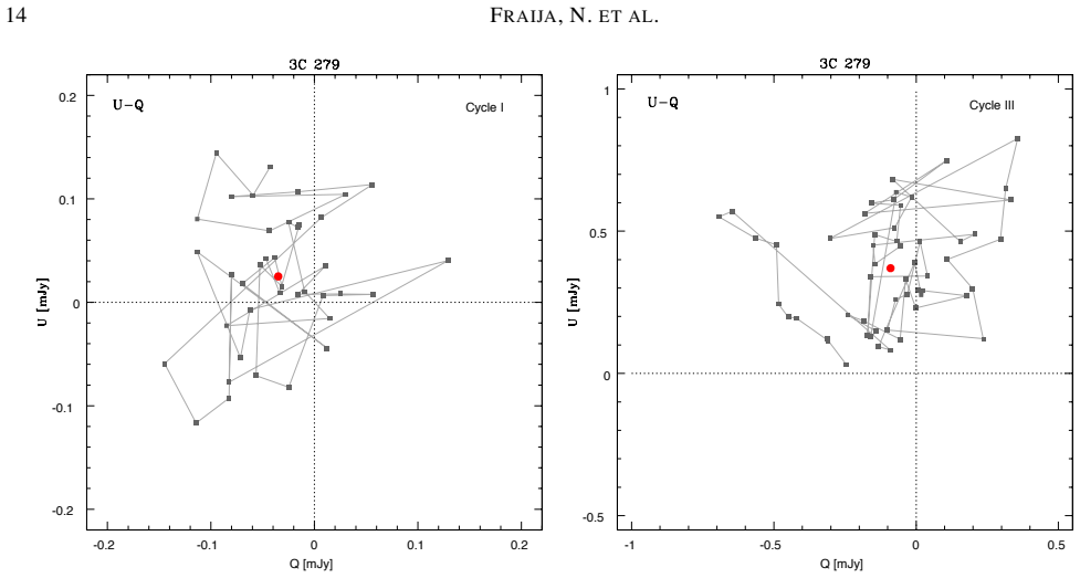
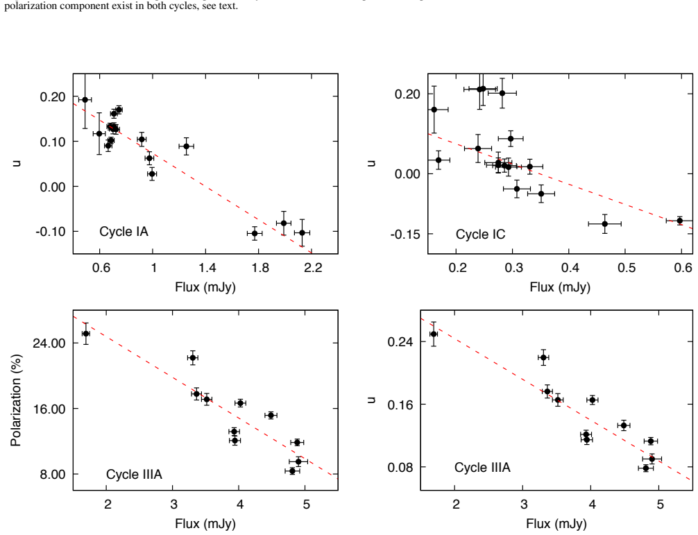
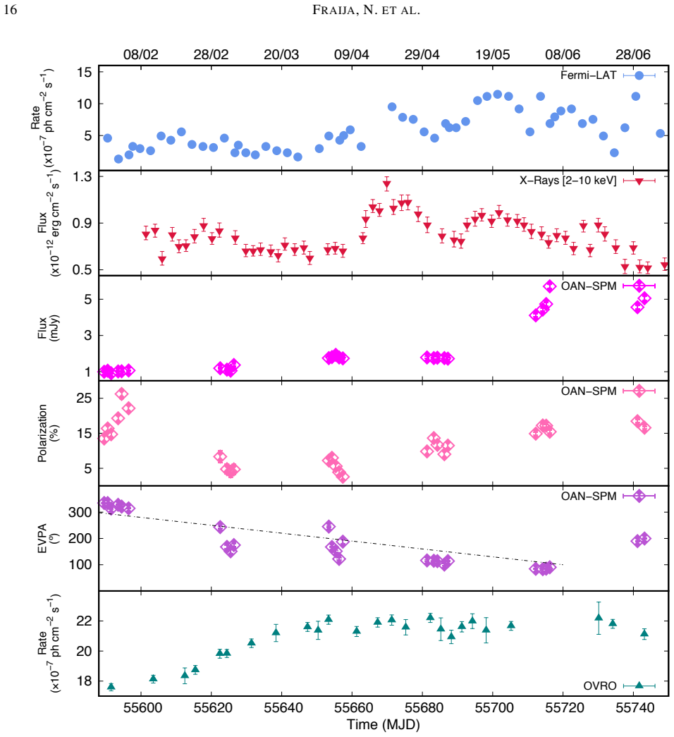
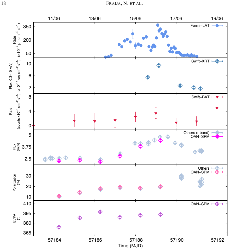
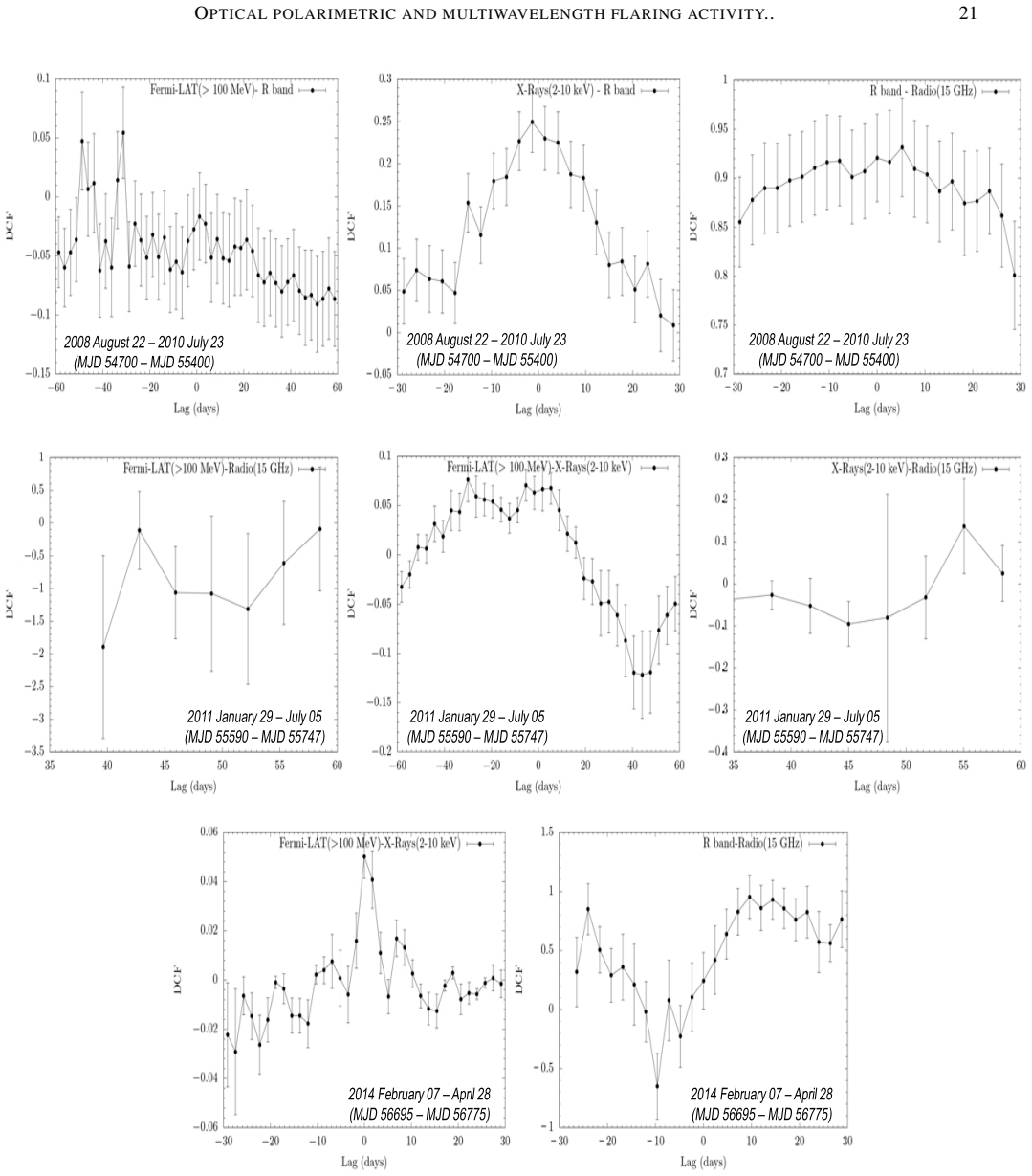
The central claim is that the large rotations of the EVPA in 3C 279 are not random but trace a change in jet orientation. In cycle II the EVPA swung by about $\sim 317^\circ$ during an optical outburst, and the preferred interpretation is jet precession driven by non-axisymmetric accretion, because precession naturally gives the smaller viewing angle and higher flux observed then. In cycles I and III, the Stokes $Q$--$U$ plane shows a stable polarized component with $P_c = (6.83 \pm 1.43)\%$ at EVPA $67.7^\circ \pm 2.5$ before the 2009 flare and $P_c = (13.30 \pm 0.56)\%$ at $52.6^\circ \pm 2.1$ after it; this doubling is presented as a lasting change in the magnetic-field or geometric configuration. The multiwavelength DCF analysis finds no simple simultaneity: in 2009 the gamma-ray/optical DCF peaks at about $-31$ and $-49$ days and X-ray/optical and radio/optical at about 1.4 and 5.2 days; in 2011 gamma-ray/radio, X-ray/radio, and gamma-ray/X-ray lags are about 43, 55, and 30 days; in 2014 gamma-rays and X-rays are nearly simultaneous while optical and radio lag by about 9.6 days. These lags are the evidence for multiple emission regions. The 2017 flare, with polarization degree rising from about 6% to 20% over 90 days while the EVPA stayed near $430^\circ$, has no reported counterparts in gamma-ray, X-ray, or radio bands, and the paper attributes it to synchrotron emission from a low-energy electron population.
Load-bearing premise
The analysis is built on a hand-drawn segmentation of the nine-year light curve into cycles and sub-cycles; if those boundaries are not physically meaningful, the per-cycle correlations, stable-component estimates, and the inferred precession scenario lose support.
Editorial extensions
If this is right
- If the precession interpretation is right, the EVPA swings in cycle II are a geometric effect rather than a change in the magnetic-field topology, and the larger flux in that cycle follows from the jet pointing closer to the line of sight.
- If the stable polarized component really doubled after 2009, the 2009 flare marked a lasting change in the emitting region's magnetic-field or geometric configuration, not just a transient outburst.
- The measured lags, if real, rule out a single emission zone for 3C 279 during the 2009 and 2011 flares; models must include at least two regions with different electron energies.
- The 2017 optical-only flare, if confirmed as orphan-like, requires a mechanism that accelerates low-energy electrons without producing the high-energy population that usually accompanies flares.
- The SED fits give an emitting-region radius around $\sim 10^{17}$ cm and radiative powers near equipartition, meaning the jet's energy budget is plausibly shared between particles and field.
Reading between the lines
- Extension: a formal change-point test on the EVPA and Stokes $q,u$ series could show whether the visually chosen cycle boundaries are real structures; the paper does not run such a test.
- Extension: if precession is the cause, the nine-year EVPA record may encode a precession period that could be checked against VLBI jet position-angle changes.
- Extension: the stable polarized component is treated as constant inside each cycle; fitting a model with a slowly drifting $Q$--$U$ offset would test whether the reported $P_c$ values are robust.
- Extension: the 2017 optical-only flare suggests a class of low-energy-electron flares; an archival search for similar events in other flat-spectrum radio quasars could establish how common they are.
Signed reviews
Editorial analysis
A structured set of objections, weighed in public.
Referee Report
Summary. The paper analyzes nine years (2008-2017) of optical R-band photopolarimetric observations of the flat-spectrum radio quasar 3C 279, together with multiwavelength campaigns covering five flaring episodes. The authors report extreme brightness states, a stable polarized component whose level rises from about 6% before 2009 to about 13% after, large EVPA rotations, and DCF-derived lags among gamma-ray, X-ray, optical, and radio bands. They interpret the EVPA behavior as evidence for jet precession and the DCF lags as evidence for multiple emission regions. They also fit the broadband SEDs with a one-zone SSC plus external-Compton model over seven epochs.
Significance. If the analysis were sound, the paper would provide valuable long-term polarimetric constraints on 3C 279 and support physically interesting scenarios: a persistent polarized component that changed between cycles and multi-zone emission during flares. The 9-year, 188-point R-band photopolarimetric data set is a genuine observational contribution, and the paper makes the data available in machine-readable form. However, the central interpretive claims rest on two pillars that are currently unreliable: the DCF lag analysis (which misreads nonzero-lag peaks as absence of correlation and supplies no significance levels) and the visually determined cycle segmentation. The SED fitting also contains a circular use of the variability timescale. These issues are fixable with reanalysis, but they affect the paper's main physical conclusions.
major comments (4)
- [§3.2-3.4, Fig. 10] The DCF results are interpreted incorrectly. In §3.2, peaks at approximately -31 and -49 days are taken to show that 'gamma-ray and optical bands are not correlated'; in §3.3, a gamma-ray/X-ray peak at 30.01 days is said to indicate that the bands 'are also not correlated'; in §3.4, an optical/radio lag of 9.6 days is used to conclude no correlation. A DCF peak at a nonzero lag is evidence of a delayed correlation, not of an absence of correlation. Moreover, no uncertainties, confidence intervals, or Monte Carlo significance tests are presented for any DCF peak, so it is not known whether the quoted peaks are statistically significant. Because the Conclusions explicitly use 'the analysis of the different DCFs' to claim that 3C 279 has multiple emission regions, these sections must be reanalyzed with proper lag-significance estimation and the interpretation corrected.
- [§2.1, Fig. 1, Tables 3-4] The division into cycles I, II, III and sub-cycles is made by visual inspection, following Beaklini et al. (2019), with no formal change-point test or robustness check. All per-cycle variability indices, Pearson correlations, and the stable-polarized-component estimates (Pc = 6.83% in cycle I and 13.30% in cycle III) are computed inside these hand-chosen windows. If the boundaries are not physically meaningful, the reported statistics and the inferred precession scenario lose support. The authors should justify the segmentation quantitatively (e.g., with a change-point test or a sensitivity analysis over plausible boundary choices) or clearly redraw the conclusions that depend on it.
- [§2.1.2, Table 3] The dates defining Cycle II and its sub-cycles are internally inconsistent. The text states that Cycle II spans 2012 March 12 (MJD 55998) to 2013 May 17 (MJD 56429), but Sub-cycle IIA is quoted as 2011 January 12 (MJD 55573) to 2011 July 01 (MJD 55743), which lies outside Cycle II and even outside the stated cycle boundaries. Sub-cycle IIB is given as 2012 February 19 (MJD 55976) to 2013 May 17 (MJD 56077), whose ending MJD does not match the Cycle II end (56429). Since Table 3 reports statistics for these sub-cycles, the data assignments must be reconciled and any resulting changes to the per-cycle correlation results must be applied.
- [§4, Table 5] The SED modeling contains a circular step and a lack of parameter uncertainty. The text states that the emitting radius is bounded by rd ≤ δD/(1+z) τv and that the magnetic field is estimated by equating synchrotron cooling with the variability timescale; it then reports that the best-fit models give variability timescales of 3.3-4.0 days. This uses the same variability timescale as an input and later presents a model-derived timescale as an output. The fits in Table 5 also list no uncertainties on δD, B, rd, Ne, or the power-law indices, so it is unclear which parameters are actually constrained by the SED data. The authors should break the circularity (e.g., treat τv as an independent input or leave it as a fitted parameter) and provide error estimates or confidence intervals for all fitted quantities.
minor comments (4)
- [Abstract] The abstract gives the maximum R-band brightness as 13.68 ± 0.11 mag (1.36 ± 0.20 mJy), but Table 2 and Section 2 quote (10.36 ± 0.20) mJy for the same event. The abstract value appears to be a typographical error and should be corrected.
- [Fig. 10] The DCF panels in Figure 10 are not identified with labels; the text refers to 'left-hand panel', 'middle', and 'right-hand panel' without marking them. Add visible panel labels (e.g., a, b, c) and refer to them explicitly in the text.
- [§3.2, Fig. 4 caption] The start date of the 2009 campaign is given as MJD 54590 in the text and MJD 54700 in the Figure 4 caption; both cannot be correct. Verify and harmonize all MJD-dated boundaries.
- [§2.1.2, Sub-cycle IIB] The wording 'Sub-cycle IIB: From 2012 February 19 (MJD 55976) to 2013 May 17 (MJD 56077)' includes an ending MJD that is earlier than the actual MJD of 2013 May 17 (56429); this appears to be a transcription error in either the date or the MJD.
Circularity Check
SED variability-timescale estimate recycles its own input constraint; core polarimetric analysis is empirical.
-
self definitional
[Section 4 (Modeling the Broadband Emission) and Section 5 (Conclusions)]
"electrons ... are confined inside the emitting zone of radius rd≤ δD/(1+z)τv, by a magnetic field, that is estimated by equating the synchrotron cooling and the variability timescales ... Our best models allowed to estimate that variability timescales are in the range of 3.3 to 4.0 days."
The variability timescale τv enters Section 4 as the quantity that sets the emitting-radius inequality rd ≤ δD/(1+z)τv and that fixes B through the synchrotron-cooling equality. The SED fits then return δD = 14–18 and rd = (1.1–2.1)×10^17 cm (Table 5). Plugging those outputs back into rd = δD c τv/(1+z) gives τv ≈ 3–4 days, which is exactly the range reported in the Conclusions. The 'estimated' variability timescale is therefore not an independent model prediction; it is the same constraint that was used to define B and rd, re-expressed. The paper does not compare this output to an independently measured variability timescale.
full rationale
The paper's main photopolarimetric results—the 9-year light curves, variability indices, per-cycle Pearson correlations, the stable component inferred from the mean of absolute Stokes parameters, and the DCF lags—are direct empirical reductions of the reported observations. They do not assume the precession scenario or the multiple-region conclusion, so those headline claims are not circular. The DCF statements that nonzero lags mean 'not correlated' are an inferential error, not a circular reduction. The subjective cycle segmentation follows Beaklini et al. (2019) and is a modeling choice, not a circularity. The only construction loop I can exhibit is in Sections 4–5: τv is used to bound rd and to fix B by equating synchrotron cooling with the variability timescale, and then τv = 3.3–4.0 days is reported as a best-model estimate; this re-expresses the input constraint rather than testing it. Because this loop concerns a secondary SED consistency check, not the paper's central claims, the overall circularity is modest.
Assumptions & free parameters
free parameters (6)
- Doppler factor delta_D =
14-18
- Magnetic field B =
0.14-2.5 G
- Emitting radius rd =
1.1-2.1 x 10^17 cm
- Electron density Ne =
0.1-0.26 x 10^3 cm^-3
- Power-law indices p1, p2, p3 =
1-6.1
- Sub-cycle boundaries =
MJD intervals
assumptions (6)
- standard math The discrete correlation function (Edelson & Krolik 1988) is a valid estimator of lags for this unevenly sampled dataset.
- domain assumption The one-zone SSC model with external Compton seed photons from BLR and IR dust describes the emission region.
- domain assumption The viewing angle is 2 degrees, gamma_min = 10, and the torus temperature is 850 K.
- ad hoc to paper The mean absolute Stokes parameters <Q> and <U> in a cycle represent a stable polarized emission component.
- domain assumption Xi_BLR = 0.2 and Xi_IR = 0.4 from Zheng & Yang (2016) are appropriate for 3C 279.
- ad hoc to paper The division into cycles I, II, III follows Beaklini et al. (2019) and is adequate for the statistical analysis.
Cite this review
Pith. "Pith review of Optical polarimetric and multiwavelength flaring activity of blazar 3C279." pith.science (2026). https://pith.science/paper/FYLCEQWK
@misc{pith2026190808663,
  author       = {Pith},
  title        = {Pith review of: Optical polarimetric and multiwavelength flaring activity of blazar 3C279},
  year         = {2026},
  howpublished = {\url{https://pith.science/paper/FYLCEQWK}},
  note         = {Machine review of arXiv:1908.08663}
}
abstract
An exhaustive analysis of 9-year optical R-band photopolarimetric data of the flat-spectrum radio quasar 3C279 from 2008 February 27 to 2017 May 25 is presented, alongside with multiwavelength observing campaigns performed during the flaring activity exhibited in 2009 February/March, 2011 June, 2014 March/April, 2015 June and 2017 February. In the R-band, this source showed the maximum brightness state of $13.68\pm 0.11$ mag ($1.36\pm0.20$ mJy) on 2017 March 02, and the lowest brightness state ever recorded of $18.20\pm 0.87$ mag ($0.16\pm0.03$ mJy) on 2010 June 17. During the entire period of observations, the polarization degree varied between $0.48\pm0.17$% and $31.65\pm0.77$% and the electric vector position angle exhibited large rotations between $82.98^\circ \pm0.92$ and $446.32^\circ \pm1.95$. Optical polarization data show that this source has a stable polarized component that varied from $\sim$6% (before the 2009 flare) to $\sim$13% after the flare. The overall behavior of our polarized variability data supports the scenario of jet precessions as responsible of the observed large rotations of the electric vector position angle. Discrete correlation function analysis show that the lags between gamma-rays and X-rays compared to the optical R-band fluxes are $\Delta t \sim$ 31 d and $1$ d in 2009. Lags were also found among gamma-rays compared with X-rays and radio of $\Delta t \sim$ 30 d and $43$ d in 2011, and among radio and optical-R band of $\Delta t \sim$ 10 d in 2014. A very intense flare in 2017 was observed in optical bands with a dramatic variation in the polarization degree (from $\sim$ 6% to 20%) in 90 days without exhibiting flaring activity in other wavelengths.
Figures

Figures from the paper (7 more)




Reference graph
Works this paper leans on
-
[1]
A., Ackermann , M., Ajello , M., et al
Abdo , A. A., Ackermann , M., Ajello , M., et al. 2010, , 463, 919
work page 2010
- [2]
-
[3]
Beaklini , P. P. B., Dominici , T. P., Abraham , Z., & Motter , J. C. 2019, , 626, A78
work page 2019
-
[4]
Beckmann , V., & Shrader , C. R. 2012, Active Galactic Nuclei
2012
- [5]
- [6]
-
[7]
Boettcher , M., & Baring , M. G. 2019, arXiv e-prints, arXiv:1903.12381
work page Pith review arXiv 2019
-
[8]
Bonning , E., Urry , C. M., Bailyn , C., et al. 2012, , 756, 13
work page 2012
Show all 56 references
-
[9]
2018, arXiv e-prints, arXiv:1807.04046
Bottacini , B \"o ttcher , M., Pian , E., Collmar , W., & Gasparrini , D. 2018, arXiv e-prints, arXiv:1807.04046
2018 arXiv
-
[10]
B \"o ttcher , M., Reimer , A., & Marscher , A. P. 2009, , 703, 1168
2009
-
[11]
2013, , 768, 54
B \"o ttcher , M., Reimer , A., Sweeney , K., & Prakash , A. 2013, , 768, 54
2013
-
[12]
A., & Krolik , J
Edelson , R. A., & Krolik , J. H. 1988, , 333, 646
1988
-
[13]
2014, , 783, 44
Fraija , N. 2014, , 783, 44
2014
-
[14]
2015, Astroparticle Physics, 71, 1
---. 2015, Astroparticle Physics, 71, 1
2015
-
[15]
Fraija , N., Aguilar-Ruiz , E., Galv \'a n-G \'a mez , A., Marinelli , A., & de Diego , J. A. 2018, , 481, 4461
2018
-
[16]
2015, Astroparticle Physics, 70, 54
Fraija , N., & Marinelli , A. 2015, Astroparticle Physics, 70, 54
2015
-
[17]
2016, , 830, 81
---. 2016, , 830, 81
2016
-
[18]
2017 a , Astroparticle Physics, 89, 14
Fraija , N., Marinelli , A., Galv \'a n-G \'a mez , A., & Aguilar-Ruiz , E. 2017 a , Astroparticle Physics, 89, 14
2017
-
[19]
2017 b , , 232, 7
Fraija , N., Ben \' tez , E., Hiriart , D., et al. 2017 b , , 232, 7
2017
-
[20]
C., Bertsch , D
Hartman , R. C., Bertsch , D. L., Fichtel , C. E., et al. 1992, , 385, L1
1992
-
[21]
C., Bertsch , D
Hartman , R. C., Bertsch , D. L., Bloom , S. D., et al. 1999, , 123, 79
1999
-
[22]
C., B \"o ttcher , M., Aldering , G., et al
Hartman , R. C., B \"o ttcher , M., Aldering , G., et al. 2001, , 553, 683
2001
-
[23]
M., Nalewajko , K., et al
Hayashida , M., Madejski , G. M., Nalewajko , K., et al. 2012, , 754, 114
2012
-
[24]
M., et al
Hayashida , M., Nalewajko , K., Madejski , G. M., et al. 2015, , 807, 79
2015
-
[25]
Heidt , J., & Wagner , S. J. 1996, , 305, 42
1996
-
[26]
2017, The Astronomer's Telegram, No
Jankowsky , F., Glawion , D., Schwemmer , S., & Wagner , S. 2017, The Astronomer's Telegram, No. 10161, 10161
2017
-
[27]
A., Lindfors , E., et al
Jermak , H., Steele , I. A., Lindfors , E., et al. 2016, , 462, 4267
2016
-
[28]
W., Rudnick , L., Aller , H
Jones , T. W., Rudnick , L., Aller , H. D., et al. 1985, , 290, 627
1985
-
[29]
2017, The Astronomer's Telegram, No
Jorstad , S., & Savchenko , S. 2017, The Astronomer's Telegram, No. 10121, 10121
2017
-
[30]
G., et al
Kiehlmann , S., Savolainen , T., Jorstad , S. G., et al. 2016, , 590, A10
2016
-
[31]
J., & Clavel , J
Klaas , U., Laureijs , R. J., & Clavel , J. 1999, , 512, 157
1999
-
[32]
M., Jorstad , S
Larionov , V. M., Jorstad , S. G., Marscher , A. P., et al. 2008, , 492, 389
2008
-
[33]
R., Stockton , A
Lynds , C. R., Stockton , A. N., & Livingston , W. C. 1965, , 142, 1667
1965
-
[34]
Marcha , M. J. M., Browne , I. W. A., Impey , C. D., & Smith , P. S. 1996, , 281, 425
1996
-
[35]
Marscher , A. P. 2014, , 780, 87
2014
-
[36]
P., Jorstad , S
Marscher , A. P., Jorstad , S. G., D'Arcangelo , F. D., et al. 2008, , 452, 966
2008
-
[37]
P., Jorstad , S
Marscher , A. P., Jorstad , S. G., Larionov , V. M., et al. 2010, , 710, L126
2010
-
[38]
2010, International Journal of Modern Physics D, 19, 701
Nalewajko , K. 2010, International Journal of Modern Physics D, 19, 701
2010
-
[39]
2018, The Astronomer's Telegram, 11239
Naurois , M. 2018, The Astronomer's Telegram, 11239
2018
-
[40]
S., Sahayanathan , S., & Stalin , C
Paliya , V. S., Sahayanathan , S., & Stalin , C. S. 2015, , 803, 15
2015
-
[41]
2017, , 467, L16
Petropoulou , M., Nalewajko , K., Hayashida , M., & Mastichiadis , A. 2017, , 467, L16
2017
-
[42]
2018, , 856, 99
Pittori , C., Lucarelli , F., Verrecchia , F., et al. 2018, , 856, 99
2018
-
[43]
J., Britzen , S., Krichbaum , T
Qian , S. J., Britzen , S., Krichbaum , T. P., & Witzel , A. 2019, , 621, A11
2019
-
[44]
G., & Marscher , A
Rani , B., Jorstad , S. G., & Marscher , A. P. 2018 a , arXiv e-prints, arXiv:1805.04588
2018 arXiv
-
[45]
G., Marscher , A
Rani , B., Jorstad , S. G., Marscher , A. P., et al. 2018 b , , 858, 80
2018
-
[46]
D., et al
Rani , B., Zhang , H., Hunter , S. D., et al. 2019, arXiv e-prints, arXiv:1903.04607
2019 arXiv
-
[47]
L., Max-Moerbeck , W., Pavlidou , V., et al
Richards , J. L., Max-Moerbeck , W., Pavlidou , V., et al. 2011, , 194, 29
2011
-
[48]
Sikora , M., Stawarz , ., Moderski , R., Nalewajko , K., & Madejski , G. M. 2009, , 704, 38
2009
-
[49]
J., Sundelius , B., & Byrd , G
Sillanp \"a \"a , A., Haarala , S., Valtonen , M. J., Sundelius , B., & Byrd , G. G. 1988, , 325, 628
1988
-
[50]
2014, , 794, 54
Sorcia , M., Ben \' tez , E., Hiriart , D., et al. 2014, , 794, 54
2014
-
[51]
2013, , 206, 11
---. 2013, , 206, 11
2013
-
[52]
S., & Miller , H
Turner , C. S., & Miller , H. R. 2017, The Astronomer's Telegram, No. 10188, 10188
2017
-
[53]
J., & Witzel , A
Wagner , S. J., & Witzel , A. 1995, , 33, 163
1995
-
[54]
C., Ramsey , B., O'Dell , S., et al
Weisskopf , M. C., Ramsey , B., O'Dell , S., et al. 2016, in , Vol. 9905, Space Telescopes and Instrumentation 2016: Ultraviolet to Gamma Ray, 990517
2016
-
[55]
2015, , 804, 58
Zhang , H., Chen , X., B \"o ttcher , M., Guo , F., & Li , H. 2015, , 804, 58
2015
-
[56]
G., & Yang , C
Zheng , Y. G., & Yang , C. Y. 2016, , 457, 3535
2016
Reviewed August 14, 2026 · model on record in the stance chip above.
Discussion (0). Continue with ORCID to comment.