REVIEW 3 major objections 4 minor 52 references
Accelerating proximal Markov chain Monte Carlo by using an explicit stabilised method
T0 review · 3 major / 4 minor · reviewed 2026-08-14 · deepseek-v4-flash
Pith's one-line read This paper claims that replacing the Euler-Maruyama discretisation in proximal MCMC with an explicit stabilised Runge-Kutta-Chebyshev (SK-ROCK) approximation speeds up sampling from ill-conditioned log-concave imaging posteriors: for…
desk verdict Genuinely useful proximal MCMC method with convincing experiments, but the O(√κ) theory in Section 3.1.1 is not proven as written and needs a correction. read the letter →
The pith
A machine-rendered reading of the paper's core claim, the machinery that carries it, and where it could break.
The reading
What carries the argument
The central object is the stochastic orthogonal Runge-Kutta-Chebyshev (SK-ROCK) integrator: an explicit $s$-stage Runge-Kutta method whose coefficients are generated from Chebyshev polynomials of the first and second kind, applied to the Moreau-Yosida smoothed Langevin diffusion. Each stage evaluates the gradient $\nabla \log \pi_\lambda(x) = -\nabla f(x) - \frac{1}{\lambda}(x - \mathrm{prox}^\lambda_g(x))$ at extrapolated points, and the scalar Gaussian analysis reduces the integrator to the recurrence $X_{n+1} = R_1(z)X_n + \sqrt{2\delta}R_2(z)\xi_{n+1}$ with $R_1(z) = T_s(\omega_0+\omega_1 z)/T_s(\omega_0)$ and $R_2(z) = U_{s-1}(\omega_0+\omega_1 z)/U_{s-1}(\omega_0)(1 + \omega_1 z/2)$. The stability region of the method grows like $s^2$, so the maximum stable stepsize $\delta^{\max}_s = l_s/(L_f + 1/\lambda)$ is much larger than MYULA's; choosing $s \approx \sqrt{\eta/2}(\kappa-1)$ stages makes the contraction constant $C = \max_i R_1(z_i)^2$ approximately $((\sqrt{\kappa}-1)/(\sqrt{\kappa}+1))^2$. This explicit stabilisation is what converts the $O(\kappa)$ gradient-evaluation complexity of Euler-Maruyama into $O(\sqrt{\kappa})$.
What would settle it
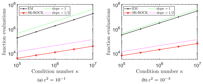
Run a controlled Gaussian experiment with known condition number $\kappa$ over several values of $\kappa$, count gradient evaluations until the empirical 2-Wasserstein distance to the exact target falls below $\varepsilon$, and compare the growth rate with $\sqrt{\kappa}$. If the count grows like $\kappa$ rather than $\sqrt{\kappa}$, or if direct evaluation of $\max_i R_1(z_i)^2$ for the recommended $s$ from equation (3.7) disagrees with $((\sqrt{\kappa}-1)/(\sqrt{\kappa}+1))^2$, the paper's central complexity claim is wrong.
Extended reading notes
Core claim
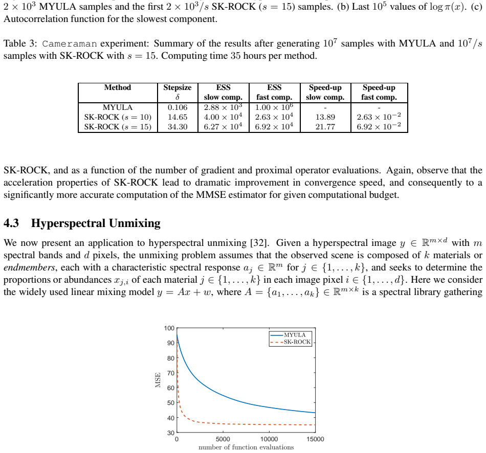
The discovery is that the stability limitation of the Moreau-Yosida unadjusted Langevin algorithm (MYULA) is not intrinsic to proximal MCMC: it is an artefact of the Euler-Maruyama discretisation. By using the SK-ROCK integrator on the same smoothed Langevin diffusion, the admissible stepsize grows roughly quadratically with the number of stages $s$, so the chain can move meaningfully along slow directions without becoming unstable along fast ones. For a Gaussian target with condition number $\kappa$, the paper derives an explicit bound $W_2(\pi, Q_n)^2 \leq W_2(\pi, \tilde{\pi})^2 + C^n W_2(\tilde{\pi}, Q_0)^2$ for the numerical chain, with $C \approx ((\sqrt{\kappa}-1)/(\sqrt{\kappa}+1))^2$, and concludes that the gradient-evaluation count to reach accuracy $\varepsilon$ is $O(\sqrt{\kappa})$ when the bias term is dominated by the contraction term. Empirically, at equal numbers of gradient and proximal evaluations, SK-ROCK with $s=10$ to $15$ outperforms MYULA by factors of $21.77$ and $37.93$ in the effective sample size of the slowest mixing component in the cameraman deconvolution and hyperspectral unmixing experiments, and reaches the typical set of the posterior far more quickly.
Load-bearing premise
The claimed $\sqrt{\kappa}$ speed-up rests on a particular formula for how fast the Chebyshev chain contracts on Gaussian targets, and on the assumption that the bias from the numerical invariant distribution is negligible compared with the target accuracy; if that formula or that negligibility fails, the $\sqrt{\kappa}$ bound fails with it.
Editorial extensions
If this is right
- For strongly log-concave imaging models, the method permits stepsizes far above MYULA's stability limit at the same number of gradient evaluations, so chains mix much faster and posterior variance estimates become usable at practical budgets.
- Under the paper's Gaussian analysis, the gradient-evaluation count for moderate accuracy scales as $O(\sqrt{\kappa})$ instead of $O(\kappa)$, matching the scaling of accelerated first-order optimisation.
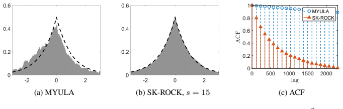
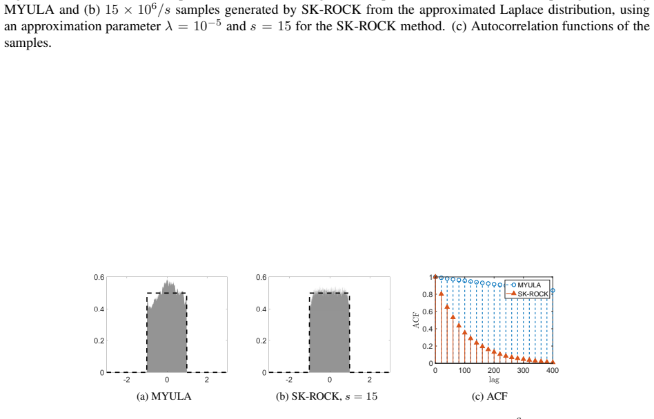
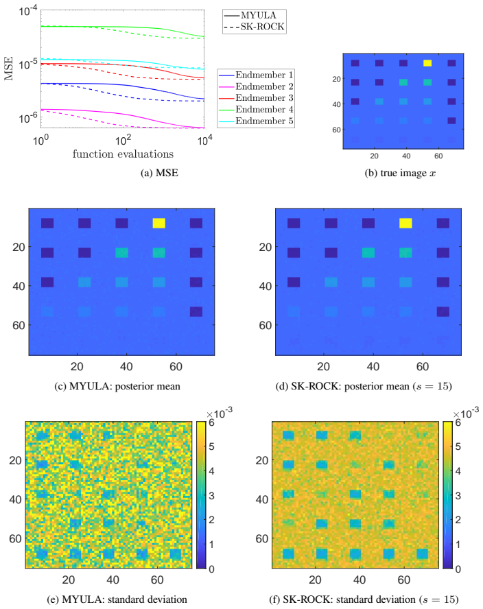
- In the reported experiments, equal-budget effective sample sizes for the slowest mixing component improve by factors of roughly 14–38 relative to MYULA, which translates directly into lower Monte Carlo variance for estimators.
- Because only the gradient and proximal oracle of MYULA is needed, the same integrator can be inserted into other proximal MCMC constructions that use MYULA as a kernel, as the authors note for future work.
- The paper recommends $s=15$ stages for strongly log-concave problems and $s=10$ otherwise, giving practitioners a simple tuning rule for imaging models.
Reading between the lines
- The paper proves the $\sqrt{\kappa}$ bound only for Gaussian targets; if the mechanism is the quadratic growth of the stability domain rather than Gaussian-specific algebra, the same qualitative acceleration should appear in other log-concave targets, but that remains a conjecture to test.
- The Wasserstein bound separates a contracted term and a bias term that is not accelerated, so the $\sqrt{\kappa}$ advantage is for moderate accuracy. A natural follow-up is a Metropolis-Hastings variant whose proposal uses the SK-ROCK step, which would remove the bias while keeping the large step.
- The method pays $s$ gradient evaluations per iteration, so the practical win depends on the cost of those evaluations relative to the proximal map; for models with expensive proximal operators, the observed effective-sample-size gains may shrink. This trade-off is not quantified in the paper.
Signed reviews
Editorial analysis
A structured set of objections, weighed in public.
Referee Report
Summary. The paper proposes a proximal Markov chain Monte Carlo method, SK-ROCK, that replaces the Euler-Maruyama discretization in the Moreau-Yosida unadjusted Langevin algorithm (MYULA) with an orthogonal Runge-Kutta-Chebyshev stochastic integrator. For Gaussian targets the authors derive an explicit Wasserstein-distance bound and claim that, under a contraction constant C approximately equal to ((sqrt(kappa)-1)/(sqrt(kappa)+1))^2, the number of gradient evaluations needed to reach a prescribed accuracy is O(sqrt(kappa)) rather than O(kappa). The method is then tested on one-dimensional Laplace and uniform targets, image deconvolution, hyperspectral unmixing, and tomographic reconstruction, with equal numbers of gradient/proximal evaluations for MYULA and SK-ROCK. The empirical sections report substantially faster autocorrelation decay, larger effective sample sizes, and lower MMSE estimation error for SK-ROCK at equal computational budget.
Significance. If the acceleration claim holds, the paper is a useful and potentially influential contribution to Bayesian imaging, since it offers a proximal MCMC algorithm that behaves like an accelerated optimization method on ill-conditioned problems. The experimental methodology is careful: comparisons are made at equal gradient-evaluation budgets, long runs are used for autocorrelation and ESS estimates, and a Metropolized P-MALA baseline is included to track asymptotic bias. The reported speedups in ESS for the slowest mixing component (21.77x and 37.93x in the cameraman and hyperspectral experiments) are striking and worth taking seriously. The Gaussian Wasserstein computation in Appendix A is self-contained and useful. However, the central theoretical complexity statement is not established by the written proof, and the paper's own formulas point to an internal inconsistency in the O(sqrt(kappa)) claim.
major comments (3)
- [Section 3.1.1, Eqs. (3.7)-(3.8)] The claim that SK-ROCK requires O(sqrt(kappa)) gradient evaluations is not supported by the displayed formulas. With delta = (omega_0 - 1)/(ell s omega_1), the slowest coordinate satisfies omega_0 + omega_1 z = 1, so R_1(z) = T_s(1)/T_s(omega_0) = 1/T_s(omega_0), giving C = max_i R_1(z_i)^2 approximately equal to cosh^{-2}(sqrt(2 eta)) = 0.907 for large kappa, which is independent of kappa and contradicts the quoted C approximately ((sqrt(kappa)-1)/(sqrt(kappa)+1))^2. Moreover, even under the quoted formula, each outer iteration costs s approximately sqrt(kappa) gradient evaluations, so O(log(epsilon^{-1}) sqrt(kappa)) outer iterations would translate to O(kappa) gradient evaluations, not O(sqrt(kappa)). Please provide a direct gradient-evaluation count from the exact Gaussian formula in Proposition 3.1, or state the complexity claim as an empirical observation.
- [Appendix B, inequality (B.1)] The proof of the key bound (3.5) uses W_2(P; Q_{n+1})^2 <= W_2(P; Qtilde)^2 + W_2(Qtilde; Q_{n+1})^2, which is not a valid use of the triangle inequality for squared 2-Wasserstein distances because the positive cross term is omitted. A correct derivation via Young's inequality would introduce an additional factor (such as 1+rho or 1+1/rho), so the displayed constant C as the sole multiplicative factor is not justified. This invalidates the non-asymptotic convergence proof as written, and therefore the complexity conclusion that rests on it.
- [Section 3.1.1, first paragraph and Proposition 3.1] The paper correctly notes that no general complexity results for Runge-Kutta-Chebyshev methods exist, and the Gaussian analysis is restricted to diagonal covariance with deterministic initial condition. The conclusion that the O(sqrt(kappa)) behavior carries over to the non-Gaussian, nonsmooth imaging models in Section 4 is therefore heuristic. Please state explicitly which parts of the theoretical claim are proved and which are conjectural, and consider adding a direct numerical check of the exact Gaussian Wasserstein formula for a range of kappa to determine whether the acceleration is genuine before the O(sqrt(kappa)) statement is presented as a theorem-level result.
minor comments (4)
- [Section 3.1.1 and Appendix A] The reference to 'Appedix A' in the text is a typo for 'Appendix A'.
- [Eq. (3.5) and Appendix B] The notation is inconsistent: the invariant measure is written as tilde pi in the main text and as tilde Q in Appendix B; please unify the notation.
- [Figure 3 and Section 3.1.1] The caption of Figure 3 mentions W_2(P; Q_0), but the precise value of Q_0 and the exact numerical procedure used to produce the curves are not given; please add enough detail to reproduce the figure.
- [Table 5] For the tomography experiment the speed-up for the fastest component is 0.81, below 1, which is not discussed; a sentence explaining why SK-ROCK can be slower on the fastest component would improve the presentation.
Circularity Check
No derivation in the paper reduces to its own inputs; the theoretical acceleration proof has a validity gap, not a circularity gap.
full rationale
The exact Wasserstein formula (Proposition 3.1 and Appendix A) is derived self-contained from the recurrence (3.2) and the definitions of R1 and R2; it is not fitting a target. The O(√κ) claim in Section 3.1.1 is not circular in the sense of equivalent-to-input: it is a claimed consequence of the contraction constant C ≈ ((√κ−1)/(√κ+1))², which the text attributes to [20] and to Appendix B. This is a minor self-citation (Zygalakis is a co-author of both the present paper and [20]), but [20] is a separate deterministic optimization theorem with stated assumptions that do not include the MCMC Wasserstein result, and the numerical comparisons are independently measured at equal gradient budgets, so the central empirical claims do not reduce to the citation. The appendix does not actually derive the C formula, and the squared triangle inequality in (B.1) is invalid, but an invalid proof is a correctness defect, not a circular redefinition or a fitted-parameter prediction. No fitted parameter is renamed as a prediction, and no self-citation is used to forbid alternatives.
Assumptions & free parameters
free parameters (4)
- Moreau-Yosida regularization λ =
0.21 (deconvolution), 7.08e-7 (hyperspectral), 0.2e-4 (tomography), 1e-5 (1D)
- Number of Chebyshev stages s =
s=15 for strong log-concavity, s=10 otherwise; s = round(sqrt(η/2)(κ−1)) in Gaussian analysis
- Damping parameter η =
0.05
- Step-size δ =
34.30 (cameraman s=15), 7.28e-7 (hyperspectral s=15), 2.30e-3 (tomography s=10)
assumptions (5)
- domain assumption The target posterior has the log-concave form π ∝ e^{-f-g} with f convex and Lipschitz differentiable and g proper, convex, and lower semicontinuous.
- domain assumption The Moreau-Yosida envelope πλ is a valid smooth approximation with Lipschitz constant Lf + 1/λ and converges to π in total variation as λ → 0.
- ad hoc to paper The Gaussian convergence analysis assumes diagonal covariance Σ and deterministic initial condition, and the bound assumes W2(π, π̃) ≪ ε so the contraction term dominates.
- standard math The SK-ROCK stability function and the contraction constant C rely on Chebyshev polynomial properties from [2] and on the formula attributed to [20], not derived in this paper.
- ad hoc to paper The scalar multiplicative-noise test equation (3.9) is representative for the mean-square stability behavior of the Langevin sampler.
Cite this review
Pith. "Pith review of Accelerating proximal Markov chain Monte Carlo by using an explicit stabilised method." pith.science (2026). https://pith.science/paper/NJ7WRMM6
@misc{pith2026190808845,
  author       = {Pith},
  title        = {Pith review of: Accelerating proximal Markov chain Monte Carlo by using an explicit stabilised method},
  year         = {2026},
  howpublished = {\url{https://pith.science/paper/NJ7WRMM6}},
  note         = {Machine review of arXiv:1908.08845}
}
abstract
We present a highly efficient proximal Markov chain Monte Carlo methodology to perform Bayesian computation in imaging problems. Similarly to previous proximal Monte Carlo approaches, the proposed method is derived from an approximation of the Langevin diffusion. However, instead of the conventional Euler-Maruyama approximation that underpins existing proximal Monte Carlo methods, here we use a state-of-the-art orthogonal Runge-Kutta-Chebyshev stochastic approximation that combines several gradient evaluations to significantly accelerate its convergence speed, similarly to accelerated gradient optimisation methods. The proposed methodology is demonstrated via a range of numerical experiments, including non-blind image deconvolution, hyperspectral unmixing, and tomographic reconstruction, with total-variation and $\ell_1$-type priors. Comparisons with Euler-type proximal Monte Carlo methods confirm that the Markov chains generated with our method exhibit significantly faster convergence speeds, achieve larger effective sample sizes, and produce lower mean square estimation errors at equal computational budget.
Figures


Figures from the paper (10 more)





Reference graph
Works this paper leans on
-
[20]
A. E FTEKHARI , B. V ANDEREYCKEN , G. V ILMART , AND K. C. Z YGALAKIS , Explicit stabilised gradient descent for faster strongly convex optimisation , arXiv e-prints, (2018)
work page 2018
-
[1]
A. A BDULLE , Explicit stabilized Runge-Kutta methods, Encyclopedia of Applied and Computational Mathemat- ics, (2015), pp. 460–468
work page 2015
-
[2]
A. A BDULLE , I. A LMUSLIMANI , AND G. V ILMART , Optimal explicit stabilized integrator of weak order one for stiff and ergodic stochastic differential equations , SIAM/ASA Journal on Uncertainty Quantification, 6 (2018), pp. 937–964
work page 2018
-
[3]
A. A BDULLE AND S. C IRILLI , S-ROCK: Chebyshev methods for stiff stochastic differenti al equations , SIAM Journal on Scientific Computing, 30 (2008), pp. 997–1014
work page 2008
-
[4]
A. A BDULLE , G. V ILMART , AND K. Z YGALAKIS , High order numerical approximation of the invariant mea- sure of ergodic sdes, SIAM Journal on Numerical Analysis, 52 (2014), pp. 1600–16 22
work page 2014
-
[5]
M. V. A FONSO , J. M. B IOUCAS -D IAS , AND M. A. T. F IGUEIREDO , Fast image recovery using variable splitting and constrained optimization , IEEE Transactions on Image Processing, 19 (2010), pp. 2345 –2356
work page 2010
-
[6]
S. A RRIDGE , P. M AASS , O. Ö KTEM , AND C.-B. S CHÖNLIEB , Solving inverse problems using data-driven models, Acta Numerica, 28 (2019), pp. 1–174
work page 2019
-
[7]
Y. A TCHADE AND A. B HATTACHARYYA , Regularization and Computation with high-dimensional spi ke-and- slab posterior distributions, arXiv e-prints, (2018), p. arXiv:1803.10282
arXiv 2018
Show all 52 references
-
[8]
B ECK , First-order methods in optimization , vol
A. B ECK , First-order methods in optimization , vol. 25 of MOS-SIAM Series on Optimization, Society for In- dustrial and Applied Mathematics (SIAM), Philadelphia, P A; Mathematical Optimization Society, Philadelphia, P A, 2017
2017
-
[9]
B ECK AND M
A. B ECK AND M. T EBOULLE , A fast iterative shrinkage-thresholding algorithm for lin ear inverse problems , SIAM Journal on Imaging Sciences, 2 (2009), pp. 183–202
2009
-
[10]
B IANCHI , A
P. B IANCHI , A. S ALIM , AND S. S CHECHTMAN , Passty Langevin, in Conference on Machine Learning (CAp) 2019, Toulouse, France, June 2019
2019
-
[11]
B ROSSE , A
N. B ROSSE , A. D URMUS , M. P EREYRA , AND E. M OULINES , Sampling from a log-concave distribution with compact support with proximal Langevin Monte Carlo , in Conference on Learning Theory (COLT) 2017, Ams- terdam, Netherlands, Sep. 2017. 25
2017
-
[12]
X. C AI, M. P EREYRA , AND J. D. M CEWEN , Uncertainty quantification for radio interferometric imag ing – I. Proximal MCMC methods, Monthly Notices of the Royal Astronomical Society, 480 (20 18), pp. 4154–4169
-
[13]
C ARMON , J
Y. C ARMON , J. C. D UCHI , O. H INDER , AND A. S IDFORD , Accelerated methods for nonconvex optimization , SIAM Journal on Optimization, 28 (2018), pp. 1751–1772
2018
-
[14]
C HAARI , J
L. C HAARI , J. T OURNERET , C. C HAUX , AND H. B ATATIA, A Hamiltonian Monte Carlo method for non-smooth energy sampling, IEEE Transactions on Signal Processing, 64 (2016), pp. 558 5–5594
2016
-
[15]
C HAMBOLLE , An algorithm for total variation minimization and applications, Journal of Mathematical imag- ing and vision, 20 (2004), pp
A. C HAMBOLLE , An algorithm for total variation minimization and applications, Journal of Mathematical imag- ing and vision, 20 (2004), pp. 89–97
2004
-
[16]
C HAMBOLLE AND T
A. C HAMBOLLE AND T. P OCK , An introduction to continuous optimization for imaging , Acta Numerica, 25 (2016), pp. 161–319
2016
-
[17]
D URMUS , S
A. D URMUS , S. M AJEWSKI , AND B. M IASOJEDOW , Analysis of Langevin Monte Carlo via convex optimiza- tion, Journal of Machine Learning Research, 20 (2019), pp. 1–46
2019
-
[18]
D URMUS AND E
A. D URMUS AND E. M OULINES , Nonasymptotic convergence analysis for the unadjusted Lan gevin algorithm, Annals of Applied Probability, 27 (2017), pp. 1551–1587
2017
-
[19]
D URMUS , E
A. D URMUS , E. M OULINES , AND M. P EREYRA , Efficient Bayesian computation by proximal Markov chain Monte Carlo: when Langevin meets Moreau , SIAM Journal on Imaging Sciences, 11 (2018), pp. 473–506
2018
-
[21]
E LSER , T
V. E LSER , T. L AN, AND T. B ENDORY , Benchmark problems for phase retrieval , SIAM Journal on Imaging Sciences, 11 (2018), pp. 2429–2455
2018
-
[22]
E LVIRA , P
C. E LVIRA , P. C HAINAIS , AND N. D OBIGEON , Bayesian antisparse coding , IEEE Transactions on Signal Processing, 65 (2017), pp. 1660–1672
2017
-
[23]
F ERNANDEZ VIDAL AND V
A. F ERNANDEZ VIDAL AND V. D E BORTOLI AND M. P EREYRA AND A. D URMUS , Maximum likelihood estimation of regularisation parameters in high-dimensional inverse problems: an empirical Bayesian approach, arXiv e-prints, (2019), p. arXiv:1911.11709
2019 arXiv
-
[24]
V EHTARI AND A
A. V EHTARI AND A. G ELMAN AND D. S IMPSON AND B. C ARPENTER AND P.C. BÃ 1 4 RKNER , Rank- normalization, folding, and localization: An improved ˆR for assessing convergence of MCMC , arXiv e-prints, (2019), p. arXiv:1903.08008
2019 arXiv
-
[25]
C. J. G EYER , Practical Markov chain Monte Carlo , Statistical Science, 7 (1992), pp. 473–483
1992
-
[26]
G IROLAMI AND B
M. G IROLAMI AND B. C ALDERHEAD , Riemann manifold Langevin and Hamiltonian Monte Carlo meth ods, Journal of the Royal Statistical Society: Series B (Statist ical Methodology), 73 (2011), pp. 123–214
2011
-
[27]
D. J. H IGHAM , A-stability and stochastic mean-square stability , BIT Numerical Mathematics, 40 (2000), pp. 404–409
2000
-
[28]
D. J. H IGHAM , Mean-square and asymptotic stability of the stochastic the ta method, SIAM Journal on Numeri- cal Analysis, 38 (2000), pp. 753–769
2000
-
[29]
H OUDARD , C
A. H OUDARD , C. B OUVEYRON , AND J. D ELON , High-dimensional mixture models for unsupervised image denoising (hdmi), SIAM Journal on Imaging Sciences, 11 (2018), pp. 2815–2846
2018
-
[30]
I ORDACHE , J
M.-D. I ORDACHE , J. M. B IOUCAS -D IAS , AND A. P LAZA , T otal variation spatial regularization for sparse hyperspectral unmixing, IEEE Transactions on Geoscience and Remote Sensing, 50 (20 12), pp. 4484–4502. 26
-
[31]
K AIPIO AND E
J. K AIPIO AND E. S OMERSALO , Statistical and computational inverse problems , vol. 160, Springer Science & Business Media, 2006
2006
-
[32]
K ESHAVA AND J
N. K ESHAVA AND J. M USTARD , Spectral unmixing, IEEE Signal Processing Magazine, 19 (2002), pp. 44–57
2002
-
[33]
P. E. K LOEDEN AND E. P LATEN , Numerical solution of stochastic differential equations, vol. 23 of Applications of Mathematics (New Y ork), Springer-V erlag, Berlin, 1992
1992
-
[34]
L UCKA , N
F. L UCKA , N. H UYNH , M. B ETCKE , E. Z HANG , P. B EARD , B. C OX, AND S. A RRIDGE , Enhancing com- pressed sensing 4d photoacoustic tomography by simultaneo us motion estimation , SIAM Journal on Imaging Sciences, 11 (2018), pp. 2224–2253
2018
-
[35]
C ORBINEAU , D
M.-C. C ORBINEAU , D. K OUAME , E. C HOUZENOUX , J.-Y. T OURNERET , AND J.-C. P ESQUET , Precondi- tioned P-ULA for Joint Deconvolution-Segmentation of Ultr asound Image , IEEE Signal Process. Letters, 26 (2019), pp. 1456–1460
2019
-
[36]
M ARNISSI , A
Y. M ARNISSI , A. B ENAZZA -B ENYAHIA , E. C HOUZENOUX , AND J. . P ESQUET , Majorize-minimize adapted metropolis-hastings algorithm. application to multichan nel image recovery, in 2014 22nd European Signal Pro- cessing Conference (EUSIPCO), Sep. 2014, pp. 1332–1336
2014
-
[37]
M ARNISSI , E
Y. M ARNISSI , E. C HOUZENOUX , J. P ESQUEI , AND A. B ENAZZA -B ENYAHIA , An auxiliary variable method for Langevin based MCMC algorithms , in 2016 IEEE Statistical Signal Processing Workshop (SSP) , June 2016, pp. 1–5
2016
-
[38]
P EREYRA , Proximal Markov chain Monte Carlo algorithms , Statistics and Computing, 26 (2016), pp
M. P EREYRA , Proximal Markov chain Monte Carlo algorithms , Statistics and Computing, 26 (2016), pp. 745– 760
2016
-
[39]
P EREYRA , Maximum-a-posteriori estimation with bayesian confidence regions, SIAM Journal on Imaging Sciences, 10 (2017), pp
M. P EREYRA , Maximum-a-posteriori estimation with bayesian confidence regions, SIAM Journal on Imaging Sciences, 10 (2017), pp. 285–302
2017
-
[40]
P EREYRA , P
M. P EREYRA , P. S CHNITER , E. C HOUZENOUX , J.-C. P ESQUET , J.-Y. T OURNERET , A. O. H ERO , AND S. M CLAUGHLIN , A survey of stochastic simulation and optimization methods in signal processing, IEEE Jour- nal of Selected Topics in Signal Processing, 10 (2016), pp. 2 24–241
2016
-
[41]
R EPETTI , M
A. R EPETTI , M. P EREYRA , AND Y. W IAUX , Scalable bayesian uncertainty quantification in imaging in verse problems via convex optimization, SIAM Journal on Imaging Sciences, 12 (2019), pp. 87–118
2019
-
[42]
R OBERT , The Bayesian choice: from decision-theoretic foundations to computational implementation , Springer Science & Business Media, 2007
C. R OBERT , The Bayesian choice: from decision-theoretic foundations to computational implementation , Springer Science & Business Media, 2007
2007
-
[43]
G. O. R OBERTS AND R. L. T WEEDIE , Exponential convergence of Langevin distributions and the ir discrete approximations, Bernoulli, 2 (1996), pp. 341–363
1996
-
[44]
R OMANO , M
Y. R OMANO , M. E LAD , AND P. M ILANFAR , The little engine that could: Regularization by denoising ( red), SIAM Journal on Imaging Sciences, 10 (2017), pp. 1804–184
2017
-
[45]
L. I. R UDIN , S. O SHER , AND E. F ATEMI , Nonlinear total variation based noise removal algorithms , Physica D: nonlinear phenomena, 60 (1992), pp. 259–268
1992
-
[46]
V ONO , N
M. V ONO , N. D OBIGEON , AND P. C HAINAIS , Sparse bayesian binary logistic regression using the split -and- augmented gibbs sampler, in 2018 IEEE 28th International Workshop on Machine Learning for Signal Processing (MLSP), Sep. 2018, pp. 1–6
2018
-
[47]
V ONO , N
M. V ONO , N. D OBIGEON , AND P. CHAINAIS , Bayesian image restoration under poisson noise and log-concave prior, in ICASSP 2019 - 2019 IEEE International Conference on Acou stics, Speech and Signal Processing (ICASSP), May 2019, pp. 1712–1716. 27
2019
-
[48]
V ONO , N
M. V ONO , N. D OBIGEON , AND P. CHAINAIS , Split-and-augmented Gibbs sampler - Application to large- scale inference problems, IEEE Transactions on Signal Processing, 67 (2019), pp. 164 8–1661
2019
-
[49]
V ONO , D
M. V ONO , D. P AULIN , AND A. D OUCET , Efficient MCMC Sampling with Dimension-Free Convergence Ra te using ADMM-type Splitting , arXiv e-prints, (2019), p. arXiv:1905.11937
2019 arXiv
-
[50]
W IBISONO , A
A. W IBISONO , A. C. W ILSON , AND M. I. J ORDAN , A variational perspective on accelerated methods in optimization, Proceedings of the National Academy of Sciences, 113 (2016 ), pp. E7351–E7358
2016
-
[51]
W IPF AND H
D. W IPF AND H. Z HANG , Revisiting bayesian blind deconvolution , Journal of Machine Learning Research, 15 (2014), pp. 3775–3814
2014
-
[52]
J. Y E, Y. H AN, AND E. C HA, Deep convolutional framelets: A general deep learning fram ework for inverse problems, SIAM Journal on Imaging Sciences, 11 (2018), pp. 991–1048. 28
2018
Reviewed August 14, 2026 · model on record in the stance chip above.
Discussion (0). Continue with ORCID to comment.