REVIEW 3 major objections 5 minor 93 references
Generative stochastic modeling of strongly nonlinear flows with non-Gaussian statistics
T0 review · 3 major / 5 minor · reviewed 2026-08-14 · deepseek-v4-flash
Pith's one-line read A data-driven framework models strongly nonlinear chaotic flows as linear stochastic oscillators seen through a nonlinear optimal-transport map, reproducing non-Gaussian statistics and heavy tails from short training data.
desk verdict A genuinely useful generative-modeling pipeline for non-Gaussian flows, but the headline tail-extrapolation claim is a model-class assumption until the transport-map degree is shown not to drive it. read the letter →
The pith
A machine-rendered reading of the paper's core claim, the machinery that carries it, and where it could break.
The reading
What carries the argument
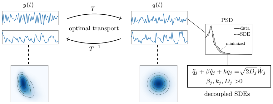
The load-bearing object is the optimal transport map $T$, taken as a lower-triangular, monotone, multivariate polynomial (a Knothe–Rosenblatt rearrangement), which pulls the data distribution back to a product reference measure, the standard normal. Because the reference measure is multiplicative, the transported coordinates $q=T(y)$ are treated as statistically independent, and each is modeled by a decoupled forced linear oscillator $\ddot q_j+\beta_j\dot q_j+k_jq_j=\sqrt{2D_j}\,\dot W_j$ whose invariant density is Gaussian; choosing $D_j=k_j\beta_j$ fixes the marginal variance, and the pair $(k_j,\beta_j)$ is optimized to match the power spectral density of $q_j$ estimated by Welch's method. The generative model is the inverse map $T^{-1}$ applied to the oscillator trajectories, so all non-Gaussianity of the data lives in the observation map rather than in the stochastic dynamics.
What would settle it
Take a two-dimensional stationary process with Gaussian marginals but nonzero lagged cross-covariance, for example two coupled Ornstein-Uhlenbeck processes; the optimal transport map is close to identity, so the fitted decoupled oscillators predict zero cross-covariance at all nonzero lags, and measuring a nonzero value in test data would falsify the decoupling assumption.
Extended reading notes
Core claim
The paper claims that a strongly nonlinear, stationary chaotic time series $y(t)\in\mathbb{R}^N$ can be modeled as $y(t)=T^{-1}(q(t))$, where $T$ is an invertible triangular polynomial map found by optimal transport from the empirical distribution of $y$ to the standard normal measure $\pi$, and each coordinate $q_j$ evolves under an independent linear stochastic oscillator $\ddot q_j+\beta_j\dot q_j+k_jq_j=\sqrt{2D_j}\,\dot W_j$, with coefficients tuned so the oscillator's power spectral density matches the spectrum of the transported coordinate. The framework therefore represents the data as a stochastic system observed through a nonlinear map, rather than fitting a nonlinear vector field. The paper demonstrates this on the Lorenz-96 system, a 10-dimensional chaotic lid-driven cavity flow at Reynolds number 30000, and reanalysis climate data, and reports that the resulting models reproduce single-point and pairwise non-Gaussian statistics, recover pointwise flow statistics from modal coordinates, and predict heavy tails from training sets far shorter than would be needed to observe those tails directly.
Load-bearing premise
The load-bearing premise is that the optimal-transport coordinates $q=T(y)$ can be treated as independent stationary Gaussian processes, so that fitting each coordinate with its own decoupled linear oscillator driven by independent white noise captures the temporal dynamics; if the true transported dynamics are dependent or non-Gaussian, the model misses lagged cross-correlations.
Editorial extensions
If this is right
- A user who has only a short time series of a chaotic, non-Gaussian system can generate much longer synthetic time series whose one-time statistics, including skewness and heavy tails, match the data.
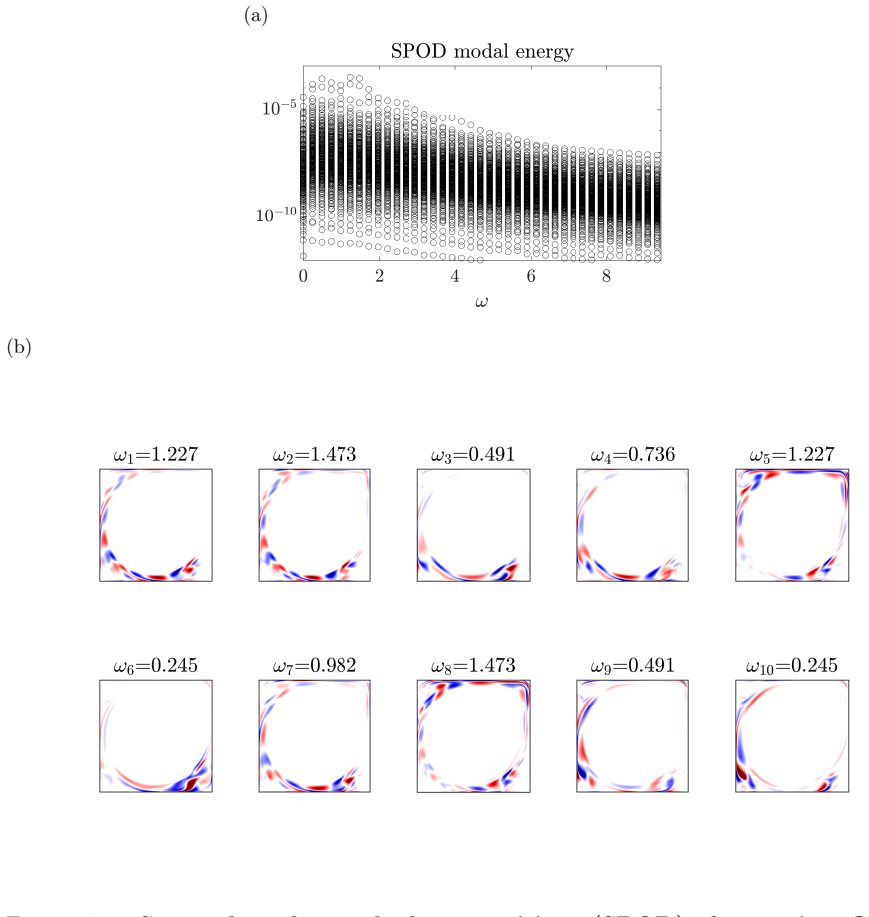
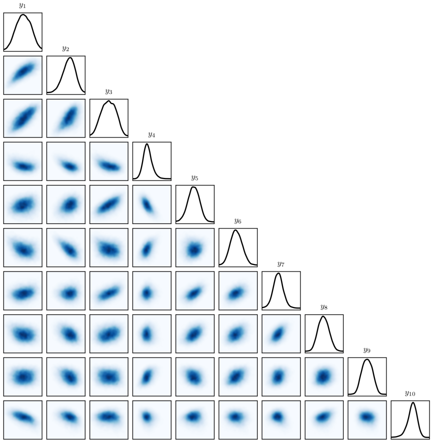
- In the cavity-flow example, fitting the model to 10 SPOD-coordinate time series yields correct marginal and pairwise joint distributions, and also recovers pointwise velocity statistics, showing that the 10-dimensional joint distribution is captured.
- The climate example shows that the model can extrapolate super-Gaussian tails of reanalysis data: a model trained on two years generates a 74-year surrogate whose tails agree with 37 years of truth.
- Because each transported coordinate is fitted independently, the computational cost separates across dimensions, making the approach tractable for systems of about ten and more dimensions.
Reading between the lines
- The decoupling assumption suggests the model will underperform when the transported coordinates have strong lagged cross-correlations; extending the linear part to a vector SDE with a full cross-spectral target would test this directly.
- The same transport-to-reference-measure idea could be pushed with non-Gaussian reference measures, such as Student-t, to model even heavier tails, or with deeper compositions of triangular maps for more complex distributions.
- A practical testable extension is to apply the framework to data with known but weak non-Gaussianity and stress-test whether the tail extrapolation is calibrated, since the paper does not provide uncertainty quantification for tail estimates beyond pointwise PDF confidence bands.
Signed reviews
Editorial analysis
A structured set of objections, weighed in public.
Referee Report
Summary. The paper proposes a data-driven procedure for constructing stochastic generative models of stationary chaotic and nonlinear flows. The method first fits a triangular polynomial optimal transport map T that pushes the data distribution to a standard normal reference distribution, then fits independent linear stochastic oscillators to the transported coordinates by matching the power spectral density of each coordinate. The resulting model is a set of decoupled linear SDEs observed through the nonlinear inverse map T^{-1}. The approach is demonstrated on the Lorenz-96 system (single observable, 1000 training samples), on the first 10 SPOD coordinates of a Re=30000 lid-driven cavity flow (2500 seconds of training data), and on 6-hourly reanalysis climate fields (1981-1982 training), with emphasis on reproducing skewness, non-Gaussian marginals, and extrapolating super-Gaussian tails.
Significance. If the claims are supported, this is a practically attractive and interpretable class of generative models for non-Gaussian stationary flows: the framework is data-efficient, scales to tens of dimensions, and comes with public code and data. The Lorenz example clearly shows the failure of a quasi-periodic phase model to capture skewness, and the cavity-flow example demonstrates good one-time marginal matching in 10 dimensions, including pointwise velocity statistics. The SPOD/Koopman connection in the paper is conceptually interesting and provides a principled justification for the choice of coordinates. However, the strongest advertised capability, tail extrapolation from short training data, currently rests on a model-class assumption that is not validated, and the independence assumption on the transported coordinates is not tested. These issues are load-bearing for the paper's central claims.
major comments (3)
- [Section 3.3, Eq. (12)] The headline claim that the framework 'predict[s] super-Gaussian tails that are not readily available from little training data' is not supported as stated. The transport map T is fitted by minimizing the KL divergence in Eq. (12) against a two-year empirical distribution, which has essentially no samples in the tail region. For the degree-2 triangular polynomial map used in Section 3.3, the large-|y| behavior of T^{-1} is determined by the squared term, so the tail shape of the generated PDF is fixed by the polynomial class rather than identified by the data. A robustness study varying the polynomial degree (and, ideally, excluding the 37-year validation interval from the training period) is needed before this prediction claim can be accepted. The paper itself acknowledges in Section 4 that theoretical characterization of the transport-map bias is beyond its scope, which makes such a numerical sensitivity check a necessary part of the argument.
- [Section 2.2, Eq. (13)] The decoupled linear oscillators in Eq. (13) are driven by independent white noises, which assumes that the transported coordinates q_j are not only marginally Gaussian but also temporally independent across coordinates. The optimal transport step diagonalizes the one-time joint distribution, but it does not guarantee that the temporal dynamics decouple. The paper validates marginal PDFs and marginal PSDs (Figs. 2, 3, and 11), but it does not report lagged cross-covariances or cross-spectral coherences between different q_j. Since the framework is presented as a generative model for a stochastic process, not just for one-time marginals, this independence hypothesis needs to be tested on at least one example; if it fails, the claim should be restricted to matching one-time statistics and marginal spectra.
- [Section 3.3, Fig. 5] The validation against the 37-year reanalysis record is partly in-sample because the 1981-1982 training interval is contained in the 'truth' data, and the shaded confidence intervals for the model PDF are not shown (only those for training and truth). To support the extrapolation claim, the authors should provide a disjoint validation period (e.g., train on 1981-1990 and validate on 1991-2017), and should display pointwise uncertainty on the 74-year model PDF so that the reader can judge whether the tail agreement is within sampling error.
minor comments (5)
- [Section 4, Eq. (26)] The displayed inequality appears to have a missing parenthesis; the expression sqrt(2(E_nu[||h||^2] - E_tildenu[||h||^2] sqrt(E_nu[log(nu/tildenu)] is not parseable as written.
- [Figure 6 caption] In panel (b) of Fig. 6, the two subcaptions both read '(right)'; the first should be '(left)'.
- [Appendix A] The text says the Lorenz data are generated by integrating Eq. (18); the Lorenz system is Eq. (17), while Eq. (18) defines the observable y.
- [Section 3.3] The climate examples use polynomials of total degree 2 while the cavity-flow example uses degree 3; the manuscript should state how the degree was selected and whether the results depend on that choice.
- [Section 2.2] The spectral matching step in Eq. (16) uses particle swarm optimization but the number of particles, the number of iterations, and the sensitivity of the fitted (k_j, beta_j) parameters are not reported; please add these details for reproducibility.
Circularity Check
No significant circularity: one-point statistics are the training objective, while the spectral matching and tail extrapolation are independent outputs.
full rationale
The derivation chain is not circular. The transport map T is fitted by KL minimization in Eq. (12) to the empirical one-time distribution, so agreement of the model's one-time marginals with the training data is the optimization objective; the paper presents this as 'reproducing' statistics rather than as an independent prediction. The predictive content lies elsewhere: the oscillator parameters are fitted to the PSD of the transported variable q, not directly to the spectrum of y, so the emergent PSD of y and the pointwise velocity statistics in the cavity flow example are nontrivial outputs; and the climate tail extrapolation is generated by pulling a 74-year SDE trajectory back through T^{-1}, with training on only 1981-1982 and validation against 1981-2017 data. The self-citations are background or factual ([2], [3], [37], [53]) and are not load-bearing for the main construction, which is implemented from stated equations and external data. Section 4 explicitly concedes that 'theoretical characterization of the bias in application to strongly nonlinear flows is beyond the scope of this paper'; that is a limitation for robustness, not a circular step. No prediction or first-principles result was found to be equivalent to its inputs by construction.
Assumptions & free parameters
free parameters (4)
- Transport map polynomial coefficients (ac, ah) =
fit to data via maximum likelihood for each example
- Oscillator stiffness kj and damping βj =
Lorenz: k=26.26, β=4.73; cavity and climate: fitted per coordinate
- Polynomial degree of transport map =
3 (Lorenz, cavity), 2 (climate)
- Number of climate covariates n =
0,1,2,3,4
assumptions (6)
- domain assumption The invariant measure ν is absolutely continuous with finite second moments, guaranteeing existence of the optimal transport map to standard normal.
- standard math The linear oscillator in Eq. (13) admits the stationary Gaussian density in Eq. (14), with variance fixed to 1 by setting Dj = kj βj.
- standard math The PSD of an observable determines the Koopman operator restricted to the cyclic subspace spanned by that observable and its history.
- domain assumption The system is stationary and ergodic, so time averages over a single long trajectory converge to ensemble averages.
- ad hoc to paper The transported coordinate processes qj(t) are independent across coordinates and are Gaussian processes, so decoupled linear SDEs fully characterize their joint law.
- domain assumption For the climate data, the time series is a mixed-spectrum process, and removing Fourier modes with more than 1% of fluctuation energy isolates the chaotic part.
Cite this review
Pith. "Pith review of Generative stochastic modeling of strongly nonlinear flows with non-Gaussian statistics." pith.science (2026). https://pith.science/paper/2QFB4MPY
@misc{pith2026190808941,
  author       = {Pith},
  title        = {Pith review of: Generative stochastic modeling of strongly nonlinear flows with non-Gaussian statistics},
  year         = {2026},
  howpublished = {\url{https://pith.science/paper/2QFB4MPY}},
  note         = {Machine review of arXiv:1908.08941}
}
read the original abstract
Strongly nonlinear flows, which commonly arise in geophysical and engineering turbulence, are characterized by persistent and intermittent energy transfer between various spatial and temporal scales. These systems are difficult to model and analyze due to combination of high dimensionality and uncertainty, and there has been much interest in obtaining reduced models, in the form of stochastic closures, that can replicate their non-Gaussian statistics in many dimensions. Here, we propose a data-driven framework to model stationary chaotic dynamical systems through nonlinear transformations and a set of decoupled stochastic differential equations (SDEs). Specifically, we use optimal transport to find a transformation from the distribution of time-series data to a multiplicative reference probability measure such as the standard normal distribution. Then we find the set of decoupled SDEs that admit the reference measure as the invariant measure, and also closely match the spectrum of the transformed data. As such, this framework represents the chaotic time series as the evolution of a stochastic system observed through the lens of a nonlinear map. We demonstrate the application of this framework in Lorenz-96 system, a 10-dimensional model of high-Reynolds cavity flow, and reanalysis climate data. These examples show that SDE models generated by this framework can reproduce the non-Gaussian statistics of systems with moderate dimensions (e.g. 10 and more), and predict super-Gaussian tails that are not readily available from little training data. These findings suggest that this class of models provide an efficient hypothesis space for learning strongly nonlinear flows from small amounts of data.
Figures


Figures from the paper (8 more)





Reference graph
Works this paper leans on
-
[1]
Agresti and B
A. Agresti and B. A. Coull , Approximate is better than “exact” for interval esti- mation of binomial proportions , The American Statistician, 52 (1998), pp. 119–126
1998
-
[2]
Arbabi and I
H. Arbabi and I. Mezic , Ergodic theory, dynamic mode decomposition, and com- putation of spectral properties of the Koopman operator , SIAM Journal on Applied Dynamical Systems, 16 (2017), pp. 2096–2126
2017
-
[3]
Arbabi and I
H. Arbabi and I. Mezi ´c, Study of dynamics in post-transient flows using Koopman mode decomposition, Phys. Rev. Fluids, 2 (2017), p. 124402
2017
-
[4]
M. Arjovsky, S. Chintala, and L. Bottou , Wasserstein GAN , arXiv preprint arXiv:1701.07875, (2017)
arXiv 2017
-
[5]
Berrisford, D
P. Berrisford, D. Dee, P. Poli, R. Brugge, M. Fielding, M. Fuentes, P. Kallberg, S. Kobayashi, S. Uppala, and A. Simmons , The ERA-interim archive version 2.0 , ECMWF Report, (2011)
2011
-
[6]
Bigoni, A
D. Bigoni, A. Spantini, R. Morrison, R. M. Baptista, and Y. Marzouk , Transport Maps Software Documentation , 2015-2020. http://transportmaps.mit. edu/docs/
2015
-
[7]
Boyd and L
S. Boyd and L. Chua , Fading memory and the problem of approximating nonlinear operators with volterra series , IEEE Transactions on circuits and systems, 32 (1985), pp. 1150–1161
1985
-
[8]
Broer and F
H. Broer and F. Takens, Mixed spectra and rotational symmetry, Archive for ratio- nal mechanics and analysis, 124 (1993), pp. 13–42
1993
Show all 93 references
-
[9]
B. W. Brunton, L. A. Johnson, J. G. Ojemann, and J. N. Kutz , Extracting spatial–temporal coherent patterns in large-scale neural recordings using dynamic mode decomposition, Journal of neuroscience methods, 258 (2016), pp. 1–15
2016
-
[10]
S. L. Brunton, B. W. Brunton, J. L. Proctor, E. Kaiser, and J. N. Kutz , Chaos as an intermittently forced linear system, Nature communications, 8 (2017), p. 19
2017
-
[11]
Chattopadhyay, P
A. Chattopadhyay, P. Hassanzadeh, and D. Subramanian, Data-driven predic- tions of a multiscale lorenz 96 chaotic system using machine-learning methods: reservoir computing, artificial neural network, and long short-term memory network , Nonlinear Processes in Geophysics, 27 (2...
2020
-
[12]
N. Chen, A. J. Majda, and D. Giannakis , Predicting the cloud patterns of the madden-julian oscillation through a low-order nonlinear stochastic model , Geophysical Research Letters, 41 (2014), pp. 5612–5619
2014
-
[13]
R. R. Coifman and S. Lafon, Diffusion maps, Applied and computational harmonic analysis, 21 (2006), pp. 5–30. 31
2006
-
[14]
Coles, J
S. Coles, J. Bawa, L. Trenner, and P. Dorazio , An introduction to statistical modeling of extreme values , vol. 208, Springer, 2001
2001
-
[15]
Cvitanovi´c, R
P. Cvitanovi´c, R. Artuso, R. Mainieri, G. Tanner, and G. Vattay , Chaos: Classical and Quantum , Niels Bohr Institute, Copenhagen, 2005. ChaosBook.org
2005
-
[16]
de la Torre and J
A. de la Torre and J. Burguete , Slow dynamics in a turbulent von k´ arm´ an swirling flow, Physical Review Letters, 99 (2007), p. 054101
2007
-
[17]
Dellnitz and O
M. Dellnitz and O. Junge , On the approximation of complicated dynamical behav- ior, SIAM Journal on Numerical Analysis, 36 (1999), pp. 491–515
1999
-
[18]
, Set oriented numerical methods for dynamical systems , Handbook of dynamical systems, 2 (2002), p. 221
2002
-
[19]
DelSole, Stochastic models of quasigeostrophic turbulence, Surveys in Geophysics, 25 (2004), pp
T. DelSole, Stochastic models of quasigeostrophic turbulence, Surveys in Geophysics, 25 (2004), pp. 107–149
2004
-
[20]
J. L. Doob, Stochastic processes, vol. 7, Wiley New York, 1953
1953
-
[21]
T. A. El Moselhy and Y. M. Marzouk , Bayesian inference with optimal maps , Journal of Computational Physics, 231 (2012), pp. 7815–7850
2012
-
[22]
N. B. Erichson, S. L. Brunton, and J. N. Kutz , Compressed dynamic mode decomposition for background modeling, Journal of Real-Time Image Processing, (2016), pp. 1–14
2016
-
[23]
B. F. Farrell and P. J. Ioannou , A theory for the statistical equilibrium energy spectrum and heat flux produced by transient baroclinic waves, Journal of the atmospheric sciences, 51 (1994), pp. 2685–2698
1994
-
[24]
A. C. M. Freitas and J. M. Freitas, On the link between dependence and indepen- dence in extreme value theory for dynamical systems , Statistics & Probability Letters, 78 (2008), pp. 1088–1093
2008
-
[25]
Goodfellow, J
I. Goodfellow, J. Pouget-Abadie, M. Mirza, B. Xu, D. Warde-Farley, S. Ozair, A. Courville, and Y. Bengio, Generative adversarial nets, in Advances in neural information processing systems, 2014, pp. 2672–2680
2014
-
[26]
Govindarajan, R
N. Govindarajan, R. Mohr, S. Chandrasekaran, and I. Mezi ´c, On the ap- proximation of Koopman spectra for measure preserving transformations, arXiv preprint arXiv:1803.03920, (2018)
2018 arXiv
-
[27]
Harlim and A
J. Harlim and A. Majda, Filtering nonlinear dynamical systems with linear stochas- tic models, Nonlinearity, 21 (2008), p. 1281
2008
-
[28]
Hasselmann, Stochastic climate models part i
K. Hasselmann, Stochastic climate models part i. theory , tellus, 28 (1976), pp. 473– 485. 32
1976
-
[29]
Kaiser, B
E. Kaiser, B. R. Noack, L. Cordier, A. Spohn, M. Segond, M. Abel, G. Daviller, J. ¨Osth, S. Krajnovi ´c, and R. K. Niven , Cluster-based reduced- order modelling of a mixing layer , Journal of Fluid Mechanics, 754 (2014), pp. 365–414
2014
-
[30]
Kevrekidis, C
I. Kevrekidis, C. W. Rowley, and M. o. Williams , A kernel-based method for data-driven Koopman spectral analysis, Journal of Computational Dynamics, 2 (2015), pp. 247–265
2015
-
[31]
Khodkar and P
M. Khodkar and P. Hassanzadeh , Data-driven reduced modelling of turbulent rayleigh–b´ enard convection using dmd-enhanced fluctuation–dissipation theorem, Jour- nal of Fluid Mechanics, 852 (2018)
2018
-
[32]
D. P. Kingma and M. Welling , Auto-encoding variational bayes , arXiv preprint arXiv:1312.6114, (2013)
2013 arXiv
-
[33]
Kinsman , Wind waves: their generation and propagation on the ocean surface , Courier Corporation, 1984
B. Kinsman , Wind waves: their generation and propagation on the ocean surface , Courier Corporation, 1984
1984
-
[34]
S. Klus, P. Koltai, and C. Sch ¨utte, On the numerical approximation of the perron-frobenius and Koopman operator, arXiv preprint arXiv:1512.05997, (2015)
2015 arXiv
-
[35]
B. O. Koopman , Hamiltonian systems and transformation in hilbert space , Proceed- ings of the National Academy of Sciences, 17 (1931), pp. 315–318
1931
-
[36]
Korda and I
M. Korda and I. Mezi ´c, On convergence of extended dynamic mode decomposition to the Koopman operator , Journal of Nonlinear Science, (2017), pp. 1–24
2017
-
[37]
Korda, M
M. Korda, M. Putinar, and I. Mezi ´c, Data-driven spectral analysis of the Koop- man operator, Applied and Computational Harmonic Analysis, (2018)
2018
-
[38]
Kravtsov, D
S. Kravtsov, D. Kondrashov, and M. Ghil , Multilevel regression modeling of nonlinear processes: Derivation and applications to climatic variability , Journal of Cli- mate, 18 (2005), pp. 4404–4424
2005
-
[39]
Lasota and M
A. Lasota and M. C. Mackey , Chaos, Fractals and Noise , Springer-Verlag, New York, 1994
1994
-
[40]
Leith , Climate response and fluctuation dissipation , Journal of the Atmospheric Sciences, 32 (1975), pp
C. Leith , Climate response and fluctuation dissipation , Journal of the Atmospheric Sciences, 32 (1975), pp. 2022–2026
1975
-
[41]
Lessig, Divergence free polar wavelets for the analysis and representation of fluid flows, Journal of Mathematical Fluid Mechanics, 21 (2019), p
C. Lessig, Divergence free polar wavelets for the analysis and representation of fluid flows, Journal of Mathematical Fluid Mechanics, 21 (2019), p. 18
2019
-
[42]
Q. Li, F. Dietrich, E. M. Bollt, and I. G. Kevrekidis, Extended dynamic mode decomposition with dictionary learning: A data-driven adaptive spectral decomposition of the Koopman operator, Chaos: An Interdisciplinary Journal of Nonlinear Science, 27 (2017), p. 103111. 33
2017
-
[43]
Lucarini, D
V. Lucarini, D. Faranda, J. M. M. de Freitas, M. Holland, T. Kuna, M. Nicol, M. Todd, S. Vaienti, et al. , Extremes and recurrence in dynamical systems, John Wiley & Sons, 2016
2016
-
[44]
J. L. Lumley, Stochastic tools in turbulence , Academic Press, 1970
1970
-
[45]
Lusch, J
B. Lusch, J. N. Kutz, and S. L. Brunton , Deep learning for universal linear embeddings of nonlinear dynamics , Nature communications, 9 (2018), p. 4950
2018
-
[46]
MacCluer, Elementary functional analysis , vol
B. MacCluer, Elementary functional analysis , vol. 253, Springer Science & Business Media, 2008
2008
-
[47]
Majda, R
A. Majda, R. V. Abramov, and M. J. Grote, Information theory and stochastics for multiscale nonlinear systems , vol. 25, American Mathematical Soc., 2005
2005
-
[48]
Majda, I
A. Majda, I. Timofeyev, and E. Vanden-Eijnden, Stochastic models for selected slow variables in large deterministic systems , Nonlinearity, 19 (2006), p. 769
2006
-
[49]
A. J. Majda and J. Harlim , Physics constrained nonlinear regression models for time series, Nonlinearity, 26 (2012), p. 201
2012
-
[50]
A. J. Majda, I. Timofeyev, and E. V. Eijnden , Models for stochastic climate prediction, Proceedings of the National Academy of Sciences, 96 (1999), pp. 14687– 14691
1999
-
[51]
A. J. Majda, I. Timofeyev, and E. Vanden Eijnden, A mathematical framework for stochastic climate models , Communications on Pure and Applied Mathematics: A Journal Issued by the Courant Institute of Mathematical Sciences, 54 (2001), pp. 891– 974
2001
-
[52]
Marzouk, T
Y. Marzouk, T. Moselhy, M. Parno, and A. Spantini , Sampling via measure transport: An introduction, Handbook of Uncertainty Quantification, (2016), pp. 1–41
2016
-
[53]
Mezi´c, Spectral properties of dynamical systems, model reduction and decompositions, Nonlinear Dynamics, 41 (2005), pp
I. Mezi´c, Spectral properties of dynamical systems, model reduction and decompositions, Nonlinear Dynamics, 41 (2005), pp. 309–325
2005
-
[54]
Mezi´c, Analysis of fluid flows via spectral properties of the Koopman operator, Annual Review of Fluid Mechanics, 45 (2013), pp
I. Mezi´c, Analysis of fluid flows via spectral properties of the Koopman operator, Annual Review of Fluid Mechanics, 45 (2013), pp. 357–378
2013
-
[55]
, Koopman operator spectrum and data analysis , arXiv preprint arXiv:1702.07597, (2017)
2017 arXiv
-
[56]
Mezic, Koopman operator, geometry, and learning, arXiv preprint arXiv:2010.05377, (2020)
I. Mezic, Koopman operator, geometry, and learning, arXiv preprint arXiv:2010.05377, (2020)
2020 arXiv
-
[57]
M. A. Mohamad, W. Cousins, and T. P. Sapsis , A probabilistic decomposition- synthesis method for the quantification of rare events due to internal instabilities , Jour- nal of Computational Physics, 322 (2016), pp. 288–308. 34
2016
-
[58]
M. A. Mohamad and T. P. Sapsis , Sequential sampling strategy for extreme event statistics in nonlinear dynamical systems , Proceedings of the National Academy of Sci- ences, 115 (2018), pp. 11138–11143
2018
-
[59]
Morrison, R
R. Morrison, R. Baptista, and Y. Marzouk, Beyond normality: Learning sparse probabilistic graphical models in the non-gaussian setting , in Advances in Neural Infor- mation Processing Systems, 2017, pp. 2359–2369
2017
-
[60]
No´e and F
F. No´e and F. Nuske, A variational approach to modeling slow processes in stochastic dynamical systems, Multiscale Modeling & Simulation, 11 (2013), pp. 635–655
2013
-
[61]
S. E. Otto and C. W. Rowley, Linearly recurrent autoencoder networks for learning dynamics, SIAM Journal on Applied Dynamical Systems, 18 (2019), pp. 558–593
2019
-
[62]
M. D. Parno and Y. M. Marzouk, Transport map accelerated Markov chain Monte Carlo, SIAM/ASA Journal on Uncertainty Quantification, 6 (2018), pp. 645–682
2018
-
[63]
Pathak, B
J. Pathak, B. Hunt, M. Girvan, Z. Lu, and E. Ott, Model-free prediction of large spatiotemporally chaotic systems from data: A reservoir computing approach , Physical Review Letters, 120 (2018), p. 024102
2018
-
[64]
J. W. L. Paul F. Fischer and S. G. Kerkemeier , nek5000 Web page , 2008. http://nek5000.mcs.anl.gov
2008
-
[65]
Peherstorfer and Y
B. Peherstorfer and Y. Marzouk , A transport-based multifidelity preconditioner for Markov chain Monte Carlo , Advances in Computational Mathematics, 45 (2019), pp. 2321–2348
2019
-
[66]
P´erez-Hern´andez, F
G. P´erez-Hern´andez, F. Paul, T. Giorgino, G. De Fabritiis, and F. No ´e, Identification of slow molecular order parameters for Markov model construction , The Journal of Chemical Physics, 139 (2013), p. 07B604 1
2013
-
[67]
Peyr´e, M
G. Peyr´e, M. Cuturi, et al. , Computational optimal transport , Foundations and Trends in Machine Learning, 11 (2019), pp. 355–607
2019
-
[68]
F. Raak, Y. Susuki, and T. Hikihara , Data-driven partitioning of power networks via Koopman mode analysis, IEEE Transactions on Power Systems, 31 (2015), pp. 2799– 2808
2015
-
[69]
Raissi, P
M. Raissi, P. Perdikaris, and G. E. Karniadakis , Numerical gaussian processes for time-dependent and nonlinear partial differential equations , SIAM Journal on Sci- entific Computing, 40 (2018), pp. A172–A198
2018
-
[70]
Rico-Martinez, I
R. Rico-Martinez, I. Kevrekidis, and K. Krischer , Nonlinear system identifi- cation using neural networks: dynamics and instabilities , Neural networks for chemical engineers, (1995), pp. 409–442
1995
-
[71]
Rico-Martinez, K
R. Rico-Martinez, K. Krischer, I. Kevrekidis, M. Kube, and J. Hudson , Discrete-vs. continuous-time nonlinear signal processing of cu electrodissolution data , Chemical Engineering Communications, 118 (1992), pp. 25–48. 35
1992
-
[72]
Rigas, A
G. Rigas, A. Morgans, R. Brackston, and J. Morrison , Diffusive dynamics and stochastic models of turbulent axisymmetric wakes , Journal of Fluid Mechanics, 778 (2015)
2015
-
[73]
Rowley, I
C. Rowley, I. Mezi´c, S. Bagheri, P. Schlatter, and D. Henningson, Spectral analysis of nonlinear flows , Journal of Fluid Mechanics, 641 (2009), pp. 115–127
2009
-
[74]
W. J. Rugh , Nonlinear system theory , Johns Hopkins University Press Baltimore, 1981
1981
-
[75]
P. J. Schmid, Dynamic mode decomposition of numerical and experimental data, Jour- nal of Fluid Mechanics, 656 (2010), pp. 5–28
2010
-
[76]
P. J. Schmid, L. Li, M. Juniper, and O. Pust , Applications of the dynamic mode decomposition, Theoretical and Computational Fluid Dynamics, 25 (2011), pp. 249–259
2011
-
[77]
Singer and R
A. Singer and R. R. Coifman , Non-linear independent component analysis with diffusion maps , Applied and Computational Harmonic Analysis, 25 (2008), pp. 226– 239
2008
-
[78]
Sobczyk, Stochastic differential equations: with applications to physics and engi- neering, vol
K. Sobczyk, Stochastic differential equations: with applications to physics and engi- neering, vol. 40, Kluwer, 1991
1991
-
[79]
Spantini, D
A. Spantini, D. Bigoni, and Y. Marzouk, Inference via low-dimensional couplings, The Journal of Machine Learning Research, 19 (2018), pp. 2639–2709
2018
-
[80]
K. R. Sreenivasan, A. Bershadskii, and J. Niemela, Mean wind and its reversal in thermal convection, Physical Review E, 65 (2002), p. 056306
2002
-
[81]
Takeishi, Y
N. Takeishi, Y. Kawahara, and T. Yairi, Learning Koopman invariant subspaces for dynamic mode decomposition , in Advances in Neural Information Processing Sys- tems, 2017, pp. 1130–1140
2017
-
[82]
Towne, O
A. Towne, O. T. Schmidt, and T. Colonius , Spectral proper orthogonal decom- position and its relationship to dynamic mode decomposition and resolvent analysis , Journal of Fluid Mechanics, 847 (2018), pp. 821–867
2018
-
[83]
Villani , Optimal transport: old and new , vol
C. Villani , Optimal transport: old and new , vol. 338, Springer Science & Business Media, 2008
2008
-
[84]
Z. Y. Wan and T. P. Sapsis , Machine learning the kinematics of spherical particles in fluid flows , Journal of Fluid Mechanics, 857 (2018)
2018
-
[85]
Z. Y. Wan, P. Vlachas, P. Koumoutsakos, and T. Sapsis , Data-assisted reduced-order modeling of extreme events in complex dynamical systems , PloS one, 13 (2018), p. e0197704
2018
-
[86]
Wang, J.-L
J.-X. Wang, J.-L. Wu, and H. Xiao , Physics-informed machine learning approach for reconstructing reynolds stress modeling discrepancies based on dns data , Physical Review Fluids, 2 (2017), p. 034603. 36
2017
-
[87]
P. Welch , The use of fast fourier transform for the estimation of power spectra: a method based on time averaging over short, modified periodograms , IEEE Transactions on Audio and Electroacoustics, 15 (1967), pp. 70–73
1967
-
[88]
Wiggins , Introduction to applied nonlinear dynamical systems and chaos , vol
S. Wiggins , Introduction to applied nonlinear dynamical systems and chaos , vol. 2, Springer Science & Business Media, 2003
2003
-
[89]
M. O. Williams, I. G. Kevrekidis, and C. W. Rowley , A data-driven approx- imation of the Koopman operator: Extending dynamic mode decomposition , Journal of Nonlinear Science, 25 (2015), pp. 1307–1346
2015
-
[90]
Yeung, S
E. Yeung, S. Kundu, and N. Hodas , Learning deep neural network repre- sentations for Koopman operators of nonlinear dynamical systems , arXiv preprint arXiv:1708.06850, (2017)
2017 arXiv
-
[91]
A. Zare, M. R. Jovanovi ´c, and T. T. Georgiou , Colour of turbulence , Journal of Fluid Mechanics, 812 (2017), pp. 636–680
2017
-
[92]
Zech and Y
J. Zech and Y. Marzouk, Sparse approximation of triangular transports on bounded domains, arXiv preprint arXiv:2006.06994, (2020)
2020 arXiv
-
[93]
Zhao and D
Z. Zhao and D. Giannakis, Analog forecasting with dynamics-adapted kernels, Non- linearity, 29 (2016), p. 2888. 37
2016
Reviewed August 14, 2026 · model on record in the stance chip above.
Discussion (0). Continue with ORCID to comment.