REVIEW 3 major objections 5 minor 38 references
Density distribution of photospheric vertical electric currents in flare active regions of the Sun
T0 review · 3 major / 5 minor · reviewed 2026-08-14 · deepseek-v4-flash
Pith's one-line read Photospheric vertical electric currents in flare active regions follow a Gaussian core at low density and a power-law tail above roughly 10,000 statampere/cm^2, with the Gaussian attributed to magnetogram noise.
desk verdict Useful first systematic PDF of photospheric |j_z|; the main shape and noise conclusion look solid, but the reported breakpoint and tail index depend on an unweighted fitting procedure that should be checked. read the letter →
The pith
A machine-rendered reading of the paper's core claim, the machinery that carries it, and where it could break.
The reading
What carries the argument
The central object is the probability density function PDF(|j_z|) of the absolute photospheric vertical electric current density, estimated from vector magnetograms by applying the differential form of Ampere's circuital law. The argument is carried by three fitting models: Model 1, a Gaussian joined to a power law at a transition point; Model 2, a Gaussian joined to a Gaussian-plus-power-law; and Model 3, a kappa function with fixed shape parameter k = 0.5. The transition point in Model 1 is chosen by minimizing residuals, and a comparison of active-region histograms with histograms from quiet edge strips supplies the noise interpretation. This machinery does the work of turning raw magnetogram data into the quantitative claim that the Gaussian component is noise and the tail is physical.
What would settle it
Compute |j_z| PDFs from vector magnetograms of the same active regions with an independent noise model, such as adding synthetic noise to the magnetograms or using higher-resolution data, and check whether the Gaussian width tracks the noise level and whether a power-law tail persists when noise is subtracted; if the Gaussian width does not match the magnetogram noise or the tail vanishes under noise correction, the claimed separation into a noise Gaussian plus a physical power law would fail.
Extended reading notes
Core claim
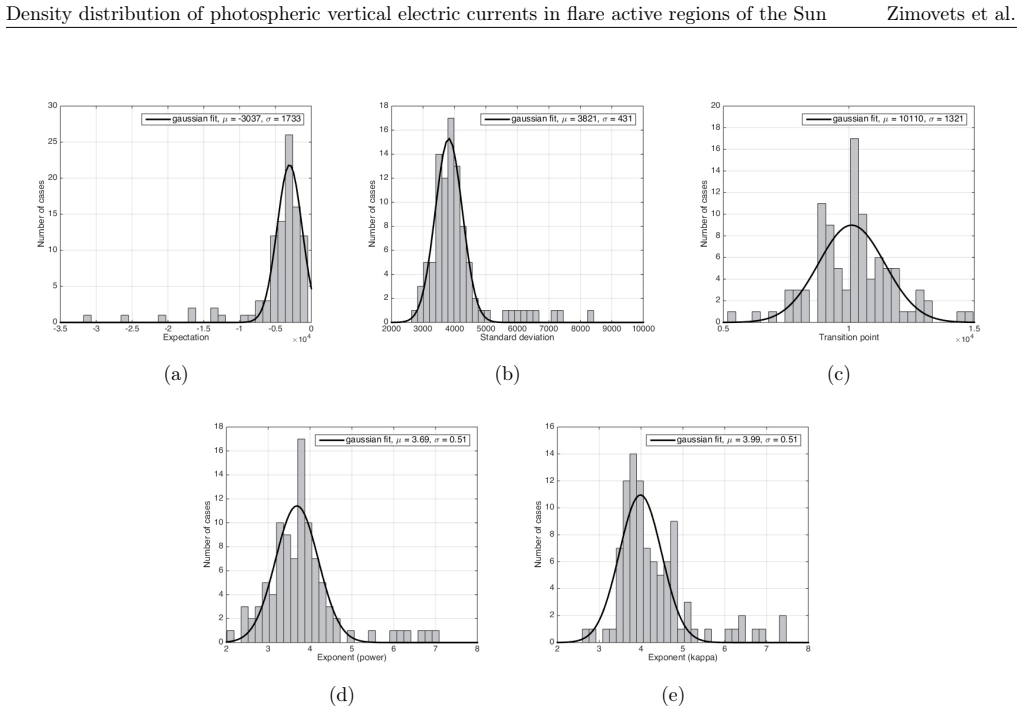
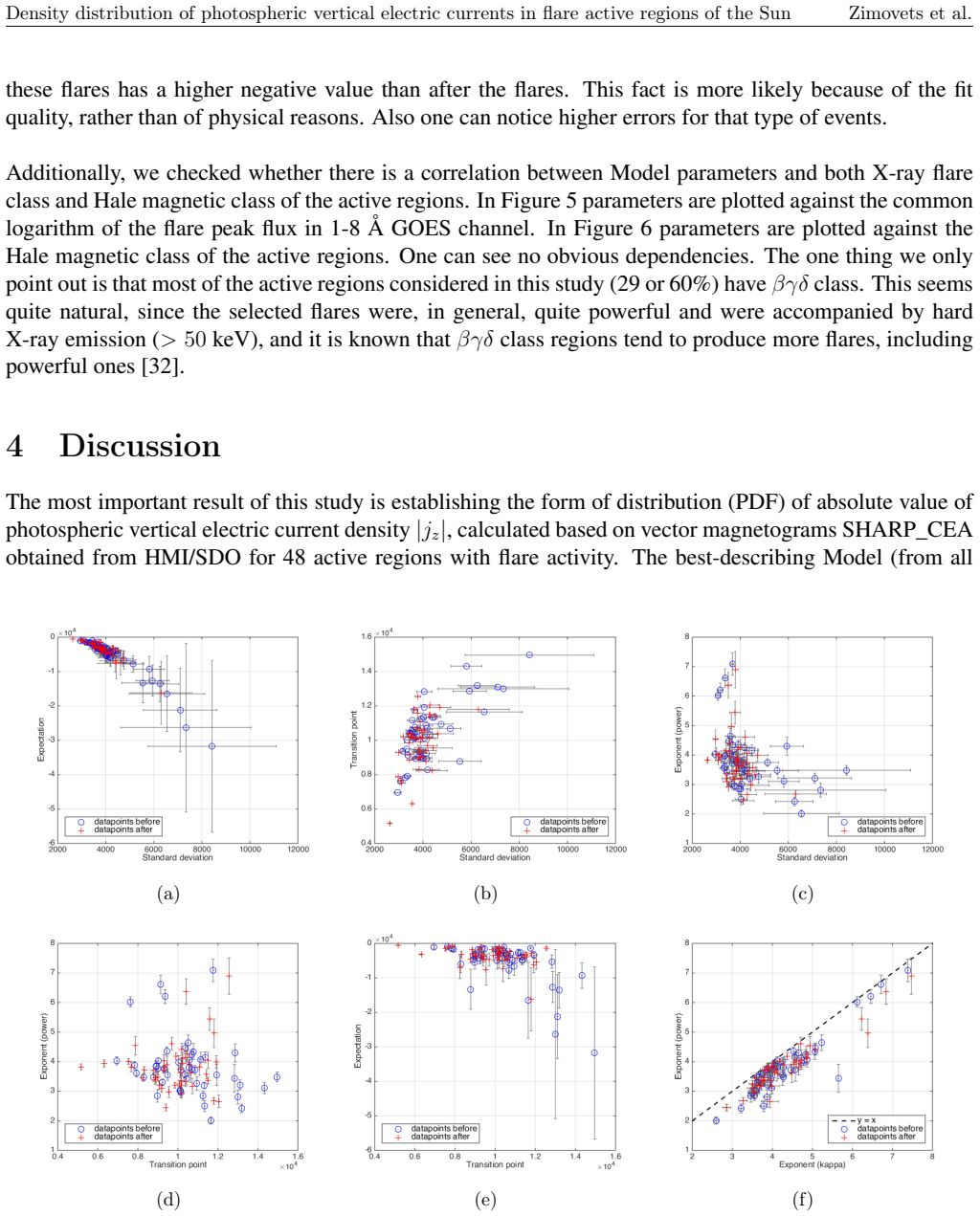
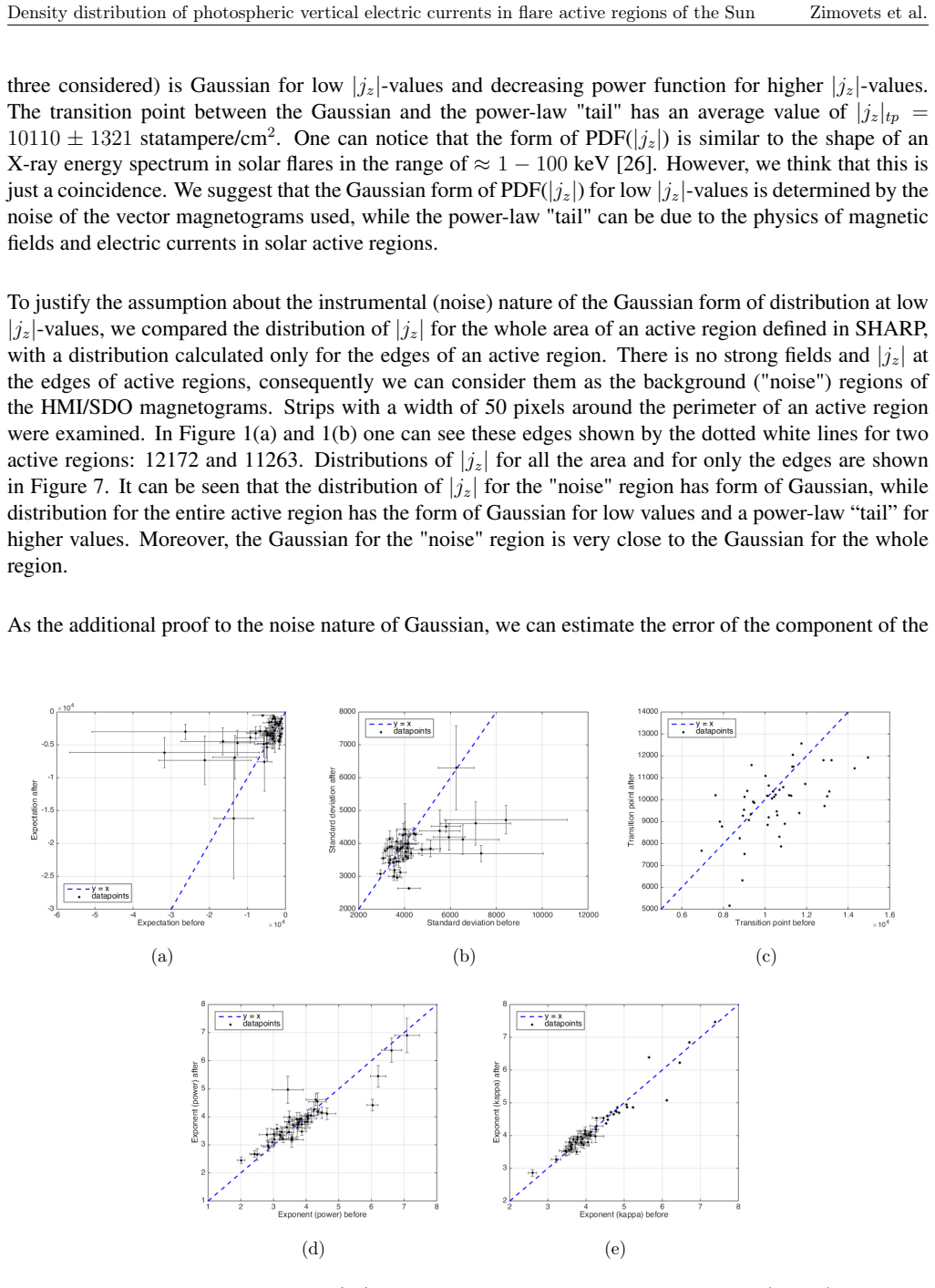
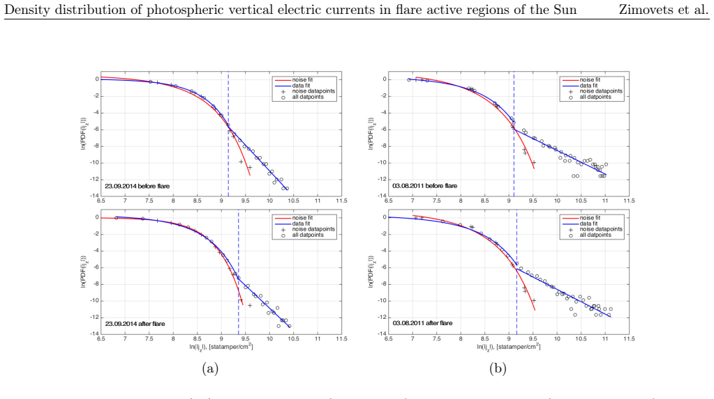
The central claim is that for the 48 flare active regions studied, the PDF of |j_z| has a two-component form: a Gaussian for |j_z| < 10110 ± 1321 statampere/$cm^{2}$ and a decaying power law above that transition, with mean absolute index 3.69 ± 0.51. For some regions the whole histogram can also be fitted by a kappa function with mean exponent 3.99 ± 0.51; the near-equality of these two exponents is taken as evidence that the high-current tail is genuinely power-law. The paper further claims that the Gaussian core is produced by noise in the vector magnetograms, supported by three observations: the |j_z| distribution in quiet edge regions is Gaussian and close to the active-region Gaussian; the Gaussian width implies a transverse-field noise of about 41 G, bracketed by the known noise levels of the magnetograph; and the transition point is close to 3σ of the fitted Gaussian. The authors find no systematic before/after flare changes in the parameters and no correlation with X-ray flare class or Hale magnetic class.
Load-bearing premise
The load-bearing premise is that fitting the histogram counts with equal weights, without accounting for Poisson or measurement uncertainties, and choosing the transition point by minimizing residuals gives unbiased values for that transition and the power-law index.
Editorial extensions
If this is right
- Current-density maps from this type of vector magnetogram should be used with a roughly 3σ cutoff (|j_z| ≈ 10,000–11,000 statampere/cm^2) to separate genuine currents from noise.
- The power-law tail, being stable across 48 active regions, gives a statistical target for models of turbulent current formation and dissipation in the photosphere.
- Global active-region averages of the current-density distribution are not sensitive markers of flare productivity; flare size and magnetic class do not change the fitted parameters.
- The near-equality of the power-law and kappa exponents means future analyses can use either functional form to characterise the tail.
- Pre- and post-flare histograms share essentially the same shape, so large-scale photospheric current systems are not rearranged by the flare itself within this sample.
Reading between the lines
- If the Gaussian core is entirely instrumental noise, the true photospheric |j_z| distribution may be a single power law extending to small values; testing this would require noise-free or higher-resolution magnetograms.
- The observed tail index of about 3.7 could be compared quantitatively with current-density PDFs from coronal magnetic-field extrapolations; a match or mismatch would test whether photospheric and coronal current statistics share a common turbulent origin.
- A testable extension is to compute PDF(|j_z|) locally, near polarity inversion lines or flare footpoints, where flare-related changes might appear even though whole-region distributions do not.
- Monitoring the tail index over many active regions might reveal correlations with flare productivity that global parameters miss.
Signed reviews
Editorial analysis
A structured set of objections, weighed in public.
Referee Report
Summary. The paper analyzes the probability density function (PDF) of the absolute value of the photospheric vertical electric current density |j_z| computed from SDO/HMI SHARP vector magnetograms for 48 flare-active regions, both before and after flares, giving 96 distributions. The authors bin |j_z| in log-log space and fit three models: a Gaussian-plus-power-law (Model 1), a Gaussian-plus-Gaussian-and-power-law (Model 2), and a kappa function (Model 3). They conclude that Model 1 best describes the data, with a Gaussian core at low |j_z| values and a decreasing power-law tail at higher values, with a mean transition point of 10110 ± 1321 statampere/cm^2 and a mean absolute power-law index of 3.69 ± 0.51. They argue that the Gaussian component represents instrumental noise, supported by an edge-region analysis and an inferred transverse-field noise of about 41 G, and that the power-law tail reflects real current structure. They report no significant flare-related changes in the parameters and no clear correlation with GOES flare class or Hale magnetic class.
Significance. If the reported shape and noise interpretation survive a more rigorous statistical treatment, the paper provides a useful empirical characterization of photospheric vertical current densities and a practical 'three-sigma' threshold for HMI-based current studies. The sample of 96 distributions is substantial, and the independent edge-region noise test plus the consistency with published HMI transverse-field noise levels are valuable falsifiable checks. The main weakness is the fitting methodology, which currently lacks error weighting and a proper treatment of the data-selected breakpoint, so the headline numbers should be regarded as provisional. No code is provided, but the underlying HMI/SHARP data are public, which helps reproducibility.
major comments (3)
- [Section 2 (Data and methods), fitting procedure] The fits are performed by unweighted nonlinear least squares on binned log-counts, with empty bins excluded and counts normalized to the maximum. Because high-|j_z| bins contain very few counts, their log-counts have large Poisson scatter, and equal weighting lets these noisy tail points disproportionately influence the power-law slope. This directly affects the central results in Table 1, namely the transition point and |f|. Please rerun the analysis with Poisson weights or a maximum-likelihood fit to the binned or unbinned data, and report per-fit parameter uncertainties from the covariance matrix.
- [Section 2 (Data and methods), transition-point selection] The breakpoint n, and hence x_tp, is chosen for each distribution by minimizing residuals. This makes the breakpoint an additional free parameter that is not penalized anywhere in the procedure. Data-selected breakpoints can bias the Gaussian and power-law parameter estimates, and the reported R2 comparisons are not a valid model-selection criterion under this procedure. Please use a profile likelihood, cross-validation, or a penalized likelihood to account for the selection, and show how the headline values in Table 1 change when this is done.
- [Section 3 and Table 1, uncertainty interpretation] The reported uncertainties, such as 10110 ± 1321 statampere/cm^2 and 3.69 ± 0.51, are the standard deviations of Gaussian fits to the histograms of the fitted parameters across the 96 distributions, not the uncertainties of individual fits. This distinction is not stated clearly. The spread mixes intrinsic active-region variation with estimation error, and readers may misinterpret the values as fit uncertainties. Please separate the two sources of scatter and state explicitly what each reported error represents.
minor comments (5)
- [Section 4 (Discussion), three-sigma argument] The statement that the transition point is similar to 3σ_stdev is not an independent test, because both quantities come from the same Model 1 fit. Please reframe this as a consistency check rather than independent evidence, or remove it in favor of the edge-region and σ(B⊥) arguments.
- [Section 2, Eq. (1)] The discretized expression for j_z has ambiguous parentheses around the terms ΔB_φ/Δθ sinθ and B_φ cosθ; please spell out the exact finite-difference scheme used so the calculation is reproducible.
- [Section 2 and Table 1] The negative value of the Gaussian mean μ for a nonnegative quantity |j_z| is striking. The authors note that fixing μ = 0 barely changes the fit, but no quantitative comparison is shown; please include this comparison, since it bears on the interpretation of the Gaussian component as noise.
- [Section 3, model comparison] The claim that Model 1 'adequately approximates data in all cases' is based on visual examination in addition to R2 thresholds. Please define quantitative acceptance criteria for visual adequacy, or base the model choice on a formal information criterion.
- [Data availability] The paper states that information about the active regions and flares will be published in a subsequent paper, but for reproducibility a table of the 48 active regions, flare times, and GOES classes should be included in an appendix or supplementary material.
Circularity Check
No significant circularity: the paper is an empirical fitting study; its noise interpretation is checked against independent edge-region and HMI calibration evidence, and no prediction is constructed from its own fitted inputs.
full rationale
The paper's central claim is a descriptive characterization: PDF(|j_z|) in 48 active regions is well fit by a Gaussian at low values and a power law at high values, with a transition around 10110 statampere/cm^2 and power-law index 3.69. These numbers are direct outputs of least-squares fits to binned histograms, not predictions derived from a theory or from the fitted parameters themselves. The transition point is selected by residual minimization and the power-law index is fitted to the tail bins; neither quantity is defined in terms of the other. The interpretation that the Gaussian component is noise is supported by two independent checks: a comparison with distributions computed only from quiet edge regions (Figure 7) and an estimate of the implied transverse-field noise sigma(B_perp) ~ 41 G, which is compared with the published HMI/SDO noise levels of 20-50 G. This is an externally falsifiable consistency test, not a circular reduction. The auxiliary comparison of |j_z|_tp with 3*sigma (10110 vs 11463 statampere/cm^2) is a consistency check between two outputs of the same fit, but it is not used to define or force either parameter. Self-citations in the paper (e.g., reference [21]) are historical or contextual and are not load-bearing for the central quantitative results. No fitted parameter is renamed as an independent prediction, and no self-citation chain is invoked to forbid alternative models. Therefore no circularity is found.
Assumptions & free parameters
free parameters (8)
- Gaussian mean µ (Model 1, per distribution) =
Average across 96 distributions: -3037 ± 1733 statampere/cm^2
- Gaussian standard deviation σ (Model 1, per distribution) =
3821 ± 431 statampere/cm^2 (average)
- Transition point |j_z|_tp (Model 1, per distribution) =
10110 ± 1321 statampere/cm^2 (average)
- Power-law exponent f (Model 1, per distribution) =
3.69 ± 0.51 (absolute value, average)
- Power-law normalization D (Model 1, per distribution) =
Not reported
- Kappa function parameters A, b, c (Model 3, per distribution) =
Exponent c/k average 3.99 ± 0.51
- Histogram bin size =
2500 statampere/cm^2
- Noise edge strip width =
50 pixels
assumptions (7)
- domain assumption Ampère's circuital law in differential form, with µ = 1, can be applied to photospheric vector magnetograms to obtain vertical current density via finite differences.
- domain assumption The SHARP_CEA vector magnetograms accurately represent the photospheric magnetic field after removal of the 180-degree ambiguity.
- ad hoc to paper Histogram counts can be modeled in log-log space with equal weights, without specifying Poisson uncertainties.
- ad hoc to paper The transition point n can be chosen by minimizing residuals, and the resulting two-group fit is a valid description of the PDF.
- domain assumption The 50-pixel edge strips of each active region represent pure noise regions of the magnetograms.
- domain assumption The positive and negative j_z distributions are symmetric, so absolute values can be combined.
- domain assumption The sample active regions are representative of flare-productive active regions.
Cite this review
Pith. "Pith review of Density distribution of photospheric vertical electric currents in flare active regions of the Sun." pith.science (2026). https://pith.science/paper/PK3HIKDQ
@misc{pith2026190809016,
  author       = {Pith},
  title        = {Pith review of: Density distribution of photospheric vertical electric currents in flare active regions of the Sun},
  year         = {2026},
  howpublished = {\url{https://pith.science/paper/PK3HIKDQ}},
  note         = {Machine review of arXiv:1908.09016}
}
abstract
Solar active regions contain electric currents. Information on the distribution of currents is important for understanding the processes of energy release on the surface of the Sun and in the overlying layers. The paper presents an analysis of the probability density function (PDF) of the absolute value of the photospheric vertical electric current density ($|j_z|$) in 48 active regions before and after flares in 2010--2017. Calculation of $|j_z|$ is performed by applying the differential form of Ampere's circuital law to photospheric vector magnetograms obtained from observations of the Helioseismic and Magnetic Imager (HMI) instrument onboard the Solar Dynamics Observatory (SDO). It has been established that for the studied active regions PDF($|j_z|$) is described by the Gauss function in the low-$|j_z|$ region ($|j_z| < 10110 \pm 1321$ statampere/cm$^2$) and the decaying power-law function in the region of higher $|j_z|$ values. Also, for some active regions PDF($|j_z|$) can be described by the special kappa-function. The distributions of the parameters of the approximating functions are obtained using the least squares method. The average absolute value of the power-law function index is $3.69 \pm 0.51$, and $3.99 \pm 0.51$ of the kappa-function. No systematic changes in parameters during the flares are detected. An explicit connection between the parameters and the flare X-ray class, as well as with the Hale magnetic class of the active regions, is not found. Arguments are presented in favor of the suggestion that the Gaussian distribution in the low-value region of PDF($|j_z|$) represents noise in the data, while the power-law "tail" reflects the nature of electric currents in the solar active regions.
Figures

Figures from the paper (4 more)


Reference graph
Works this paper leans on
-
[1]
(ed Stenflo, J.) Solar Magnetic Fields: Polarized Radiation Diagnostics 189 (Mar. 1994). doi:10.1007/978-94-015-8246-9
-
[2]
(ed Ryutova, M.) Physics of Magnetic Flux Tubes 417 (2015). doi:10 . 1007 / 978 - 3 - 662 - 45243-1
work page 2015
-
[3]
Severny, A. B. Nekotorie problemi fiziki Solnca(Moskva, Nauka, 1988)
work page 1988
-
[4]
Fleishman, G. D. & Pevtsov, A. A. Electric Currents in the Solar Atmosphere in Electric Currents in Geospace and Beyond (eds Keiling, A., Marghitu, O. & Wheatland, M.) 235 (Mar. 2018), 43–65. doi:10.1002/9781119324522.ch3
-
[5]
Puschmann, K. G., Ruiz Cobo, B. & Martı´nez Pillet, V. The Electrical Current Density Vector in the Inner Penumbra of a Sunspot.The Astrophysical Journal Letters721, L58–L61 (Sept. 2010)
work page 2010
-
[6]
Fursyak, Y. A. & Abramenko, V. I. Possibilities for Estimating Horizontal Electrical Currents in Active Regions on the Sun.Astrophysics 60, 544–552 (Dec. 2017)
work page 2017
-
[7]
Schmieder, B. & Aulanier, G.Solar Active Region Electric Currents Before and During Erup- tive Flares in Electric Currents in Geospace and Beyond(eds Keiling, A., Marghitu, O. & Wheatland, M.) 235 (Feb. 2018), 391–406. doi:10.1002/9781119324522.ch23. arXiv: 1903. 04050 [astro-ph.SR]
-
[8]
Stepanov, A. V. & Zaitsev, V. V.Magnitosferi aktivnih oblastei Solnca i zvezd(Moskva, Fiz- matlit, 2019). 12 Density distribution of photospheric vertical electric currents in flare active regions of the Sun Zimovets et al
work page 2019
Show all 38 references
-
[9]
I., Gopasiuk, S
Abramenko, V. I., Gopasiuk, S. I. & Ogir’, M. B. Identification of varieties of solar flares based on an investigation of electric currents.Izvestiya Ordena Trudovogo Krasnogo Znameni Krymskoj Astrofizicheskoj Observatorii81, 8–13 (1990)
1990
-
[10]
K., Park, S.-H
Kontogiannis, I., Georgoulis, M. K., Park, S.-H. & Guerra, J. A. Non-neutralized Electric Currents in Solar Active Regions and Flare Productivity.Solar Physics 292, 159 (Nov. 2017)
2017
-
[11]
Fursyak, Y. A. Vertical Electric Currents in Active Regions: Calculation Methods and Relation to the Flare Index.Geomagnetism and Aeronomy58, 1129–1135 (Dec. 2018)
2018
-
[12]
Moreton, G. E. & Severny, A. B. Magnetic Fields and Flares in the Region CMP 20 September
-
[13]
Romanov, V. A. & Tsap, T. T. Magnetic Fields and Flare Activity.Soviet Astronomy 34, 656 (Dec. 1990)
1990
-
[14]
I., Gopasiuk, S
Abramenko, V. I., Gopasiuk, S. I. & Ogir’, M. B. Plasma motions and electric currents in an active region. Izvestiya Ordena Trudovogo Krasnogo Znameni Krymskoj Astrofizicheskoj Observatorii 81, 3–8 (1990)
1990
-
[15]
C., de La Beaujardiere, J.-F
Canfield, R. C., de La Beaujardiere, J.-F. & Leka, K. D. Flare Energy Release: Observational Consequences and Signatures.Philosophical Transactions of the Royal Society of London Series A 336, 381–387 (Sept. 1991)
1991
-
[16]
R., Canfield, R
Li, J., Metcalf, T. R., Canfield, R. C., Wülser, J.-P. & Kosugi, T. What Is the Spatial Rela- tionship between Hard X-Ray Footpoints and Vertical Electric Currents in Solar Flares?The Astrophysical Journal 482, 490–497 (June 1997)
1997
-
[17]
& Bommier, V
Musset, S., Vilmer, N. & Bommier, V. Hard X-ray emitting energetic electrons and photo- spheric electric currents.Astronomy and Astrophysics580, A106 (Aug. 2015)
2015
-
[18]
Sharykin, I. N. & Kosovichev, A. G. Fine Structure of Flare Ribbons and Evolution of Electric Currents. The Astrophysical Journal Letters788, L18 (June 2014)
2014
-
[19]
N., Kosovichev, A
Sharykin, I. N., Kosovichev, A. G. & Zimovets, I. V. Energy Release and Initiation of a Sun- quake in a C-class Flare.The Astrophysical Journal807, 102 (July 2015)
2015
-
[20]
A., Grigoryeva, I
Livshits, M. A., Grigoryeva, I. Y., Myshyakov, I. I. & Rudenko, G. V. Evidence for a relation- ship between emerging magnetic fields, electric currents, and solar flares observed on May 10,
-
[21]
V., Sharykin, I
Zimovets, I. V., Sharykin, I. N., Wang, R., Liu, Y. D. & Kosovichev, A. G. Relationship between Hard X-Ray Footpoint Sources and Photospheric Electric Currents in Solar Flares: a Statistical Study.AGU Fall Meeting Abstracts(Dec. 2017)
2017
-
[22]
& Nishizuka, N
Kang, J., Magara, T., Inoue, S., Kubo, Y. & Nishizuka, N. Distribution characteristics of coronal electric current density as an indicator for the occurrence of a solar flare.Publications of the Astronomical Society of Japan68, 101 (Dec. 2016)
2016
-
[23]
et al.An observationally-driven kinetic approach to coronal heating.Astronomy and Astrophysics 596, A56 (Nov
Moraitis, K. et al.An observationally-driven kinetic approach to coronal heating.Astronomy and Astrophysics 596, A56 (Nov. 2016)
2016
-
[24]
E., Ellerman, F., Nicholson, S
Hale, G. E., Ellerman, F., Nicholson, S. B. & Joy, A. H. The Magnetic Polarity of Sun-Spots. The Astrophysical Journal49, 153 (Apr. 1919)
1919
-
[25]
Scherrer, P. H. et al.The Helioseismic and Magnetic Imager (HMI) Investigation for the Solar Dynamics Observatory (SDO).Solar Physics 275, 207–227 (Jan. 2012)
2012
-
[26]
P.et al.The Reuven Ramaty High-Energy Solar Spectroscopic Imager (RHESSI).Solar Physics 210, 3–32 (Nov
Lin, R. P.et al.The Reuven Ramaty High-Energy Solar Spectroscopic Imager (RHESSI).Solar Physics 210, 3–32 (Nov. 2002)
2002
-
[27]
Bobra, M. G. et al. The Helioseismic and Magnetic Imager (HMI) Vector Magnetic Field Pipeline: SHARPs - Space-Weather HMI Active Region Patches.Solar Physics 289, 3549– 3578 (Sept. 2014). 13 Density distribution of photospheric vertical electric currents in flare active regions...
2014
-
[28]
Hoeksema, J. T. et al. The Helioseismic and Magnetic Imager (HMI) Vector Magnetic Field Pipeline: Overview and Performance.Solar Physics 289, 3483–3530 (Sept. 2014)
2014
-
[29]
Calabretta, M. R. & Greisen, E. W. Representations of celestial coordinates in FITS.Astron- omy and Astrophysics395, 1077–1122 (Dec. 2002)
2002
-
[30]
Thompson, W. T. Coordinate systems for solar image data.Astronomy and Astrophysics449, 791–803 (Apr. 2006)
2006
-
[31]
M., Kosovichev, A
Sadykov, V. M., Kosovichev, A. G., Kitiashvili, I. N. & Kerr, G. S. Response of SDO/HMI observables to heating of the solar atmosphere by precipitating high-energy electrons.arXiv e-prints. arXiv: 1906.10788 [astro-ph.SR] (June 2019)
1906 arXiv
-
[32]
& Wang, H
Toriumi, S. & Wang, H. Flare-productive active regions.Living Reviews in Solar Physics16, 3 (May 2019)
2019
-
[33]
Abramenko, V. I. & Longcope, D. W. Distribution of the Magnetic Flux in Elements of the Magnetic Field in Active Regions.The Astrophysical Journal619, 1160–1166 (Feb. 2005)
2005
-
[34]
Abramenko, V. I. Relationship between Magnetic Power Spectrum and Flare Productivity in Solar Active Regions.The Astrophysical Journal629, 1141–1149 (Aug. 2005)
2005
-
[35]
& Yurchyshyn, V
Abramenko, V. & Yurchyshyn, V. Magnetic Energy Spectra in Solar Active Regions. The Astrophysical Journal 720, 717–722 (Sept. 2010)
2010
-
[36]
S., Abramenko, V
Kutsenko, A. S., Abramenko, V. I., Kuzanyan, K. M., Xu, H. & Zhang, H. Intermittency spectra of current helicity in solar active regions.Monthly Notices of the Royal Astronomical Society 480, 3780–3787 (Nov. 2018). 14
2018
-
[1963]
Solar Physics 3, 282–297 (Feb. 1968)
1968
-
[2012]
Astronomy Reports 60, 939–948 (Oct. 2016)
2016
Reviewed August 14, 2026 · model on record in the stance chip above.
Discussion (0). Continue with ORCID to comment.