REVIEW 3 major objections 4 minor 42 references
Wasserstein Gradient Flow Formulation of the Time-Fractional Fokker-Planck Equation
T0 review · 3 major / 4 minor · reviewed 2026-08-14 · deepseek-v4-flash
Pith's one-line read This paper proves that a JKO-type variational scheme for the time-fractional Fokker-Planck equation converges weakly in $L^1$ to the unique weak solution as the time step tends to zero.
desk verdict First JKO-type variational scheme for the time-fractional Fokker-Planck equation, with a mostly sound convergence proof whose stated full-sequence uniqueness result outruns the imported well-posedness. read the letter →
The pith
A machine-rendered reading of the paper's core claim, the machinery that carries it, and where it could break.
The reading
What carries the argument
The machinery is the L1 scheme for the Caputo derivative together with its weights $b^{(n)}_i$, which turn the nonlocal fractional derivative into a weighted sum over past time levels and enter the scheme through the convex combination $\bar{\rho}^{n-1} = \sum_{i=0}^{n-1}(-b^{(n)}_{n-i})\rho^i$. A discrete integration-by-parts identity (Lemma 3.3) ties the left-sided L1 derivative used in the scheme to a right-sided L1 derivative acting on test functions, and Theorem 3.1 supplies the approximation errors that allow the limit passage. Around this, energy estimates on the free energy, second moments, and summed Wasserstein distances provide the compactness needed to extract a weakly convergent subsequence and identify the limit as a weak solution of (1.1).
What would settle it
Concretely, exhibit two weak solutions of (1.1) in the sense of Definition 2.1 with the same initial datum, or verify directly whether the right-sided L1 approximant $D^\alpha_\tau \phi$ converges to $tD^\alpha_T \phi$ as $\tau\to 0$; failure of either check would break the identification of the limit as the unique weak solution.
Extended reading notes
Core claim
The central claim is Theorem 4.2: for any fixed final time $T>0$, under Assumption 4.1 on the confinement potential, the piecewise-constant interpolants $\rho_\tau$ of the minimizers of Scheme 4.1 converge, as $\tau\to 0$, weakly in $L^1((0,T)\times\mathbb{R}^d)$ to the unique weak solution $\rho$ of the time-fractional Fokker-Planck equation (1.1) in the sense of Definition 2.1. The novelty is that the memory of the Caputo derivative is encoded in the discrete scheme through the convex combination $\bar{\rho}^{n-1}$ of all previously computed densities, with weights given by the L1 quadrature for the fractional derivative; the proof passes to the limit in the Euler-Lagrange equation using energy estimates, a discrete Gronwall inequality, and compactness in $L^1$. If the theorem is correct, it supplies the analogue, for fractional-in-time Fokker-Planck equations, of the classical JKO variational principle, and it recovers the classical JKO scheme as $\alpha\to 1$.
Load-bearing premise
The load-bearing premise is that the weak solution of (1.1) in the sense of Definition 2.1 is unique, a fact imported from a formally equivalent reformulation (2.7) for which existence and uniqueness are known; if the two weak formulations do not coincide, the convergence theorem identifies the limit only up to that equivalence, and the assertion of convergence to 'the' unique solution has no independent basis.
Editorial extensions
If this is right
- The time-fractional Fokker-Planck equation gains a variational (minimizing-movement) structure, so questions about equilibria, long-time behaviour, and stability can be studied through the discrete scheme rather than only through the PDE.
- The scheme is a genuine fractional analogue of the JKO scheme and reduces to it when $\alpha\to 1$, giving a unified time-discretization family for subdiffusive and classical diffusion.
- Because each step only costs one Wasserstein minimization plus evaluation of a convex combination of past densities, the memory of the fractional derivative is captured at essentially the computational price of the classical JKO scheme.
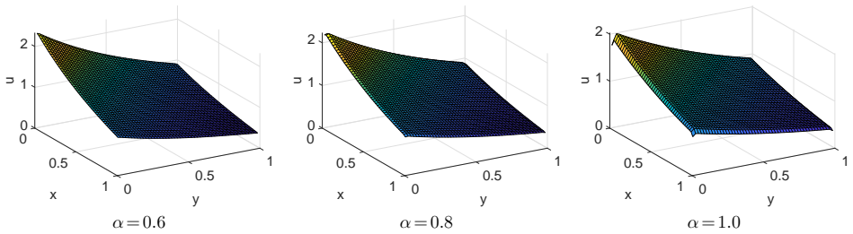
- The numerical experiments indicate sublinear convergence in $L^1$, $L^2$, and Wasserstein distance, slower than the classical first-order rate, which suggests a separate convergence-rate theory is needed for the fractional case.
- Convergence is in the weak $L^1$ sense, so further regularity of the limit would be needed to upgrade it to strong convergence or pointwise statements.
Reading between the lines
- If the formal equivalence between (1.1) and (2.7) is made rigorous, the uniqueness assumption would be fully justified; a direct well-posedness proof for Definition 2.1 would also remove the main gap in the convergence theorem and let the result stand alone.
- The proof's use of the right-sided L1 approximation, asserted but not proved, can be tested independently; establishing a symmetric error estimate would make the limit passage self-contained and likely transfer to other nonlocal-in-time gradient flows.
- The same convex-combination memory mechanism could yield JKO-type schemes for other nonlocal-in-time equations, such as Volterra-type Fokker-Planck equations with more general memory kernels, where the L1 weights would be replaced by the corresponding quadrature.
- A quantitative version of the theorem could be pursued by combining sharper L1 error estimates with regularity of the fractional Fokker-Planck solution; the empirical rates around 0.47 in Wasserstein distance provide a target for such a rate.
Signed reviews
Editorial analysis
A structured set of objections, weighed in public.
Referee Report
Summary. The paper proposes a Wasserstein gradient-flow (JKO-type) variational formulation for the time-fractional Fokker-Planck equation (1.1), where the Caputo time derivative is discretized with the L1 scheme. The discrete scheme, Scheme 4.1, replaces the immediate previous density in the classical JKO functional by a convex combination of all past densities, thereby encoding the memory of the fractional derivative. The main result, Theorem 4.2, asserts that the piecewise constant interpolants of the discrete minimizers converge weakly in L^1((0,T) x R^d) to the unique weak solution of (1.1) in the sense of Definition 2.1. The proof derives the Euler-Lagrange equation (5.17), establishes a priori estimates in Lemmas 5.3-5.5, uses a discrete integration-by-parts identity in Lemma 3.3, and passes to the limit in the discrete weak formulation. Numerical experiments in one and two dimensions illustrate the behavior of the scheme.
Significance. If the gaps identified below are repaired, this would be a valuable and novel contribution: it gives the first JKO-type variational formulation and convergent time discretization for a nonlocal-in-time Fokker-Planck equation, directly addressing a question raised by Kemppainen and Zacher. The proof strategy is sound and nearly all technical steps check out: the Euler-Lagrange equation, the a priori estimates, and the discrete integration by parts are genuinely derived and not fitted. The paper also ships a concrete computational algorithm based on entropic regularization, and the numerical section is reproducible in structure. The main theoretical claim is currently overstated because uniqueness of weak solutions in the sense of Definition 2.1 is not established within the paper, and one discrete limit used in the proof is not covered by the stated theorem. These are repairable, but they are load-bearing for the full convergence statement.
major comments (3)
- [Section 2.3 and Theorem 4.2] The assertion in Theorem 4.2 that the full sequence rho_tau converges to the unique weak solution of (1.1) in the sense of Definition 2.1 is not supported by the proof. The proof of Theorem 4.2 only shows that every subsequential L1 weak limit of the interpolants satisfies the weak formulation (2.9). Uniqueness in the class of Definition 2.1 is imported from [10, Theorem 3.3], but that theorem applies to the reformulation (2.7), and Remark 2.1 establishes equivalence of (1.1) and (2.7) only formally. Section 2.3 explicitly leaves a rigorous study of well-posedness of (1.1) to future work. If the weak-solution classes of (1.1) and (2.7) differ, different subsequences could converge to different weak solutions, and neither the word 'unique' nor the convergence of the full sequence follows. The theorem should either be weakened to subsequential convergence to a weak solution, or uniqueness for Definition 2.1 (or the equivalence of the two weak formulations) must be proved.
- [Theorem 4.2 proof and Theorem 3.1] The limit passage around Eq. (5.34) uses the convergence D_tau^alpha phi(t) -> t D_T^alpha phi(t) as tau -> 0, but Theorem 3.1 provides error estimates only for the left-sided L1 approximation dbar_tau^alpha phi and for the boundary term involving the weights b_n^(n). The right-sided discrete derivative D_tau^alpha defined in Eq. (3.12) is a symmetric analogue, and the required convergence is very likely true, but it is neither stated nor proved. Since the weak formulation (2.9) is obtained precisely from this term, the proof of Theorem 4.2 has a gap at a load-bearing step. Add an explicit error estimate or a convergence proof for the right-sided L1 approximation, along the same lines as the left-sided estimate in Theorem 3.1.
- [Lemma 5.4] The proof of the uniform second-moment bound invokes Corollary 5.1 with phi = |x|^2, but Corollary 5.1 is stated for phi in C_c^infty(R^d). The sentence 'This choice is justified by the finiteness of the second moment of each of the rho_n' is not a proof; a truncation/approximation argument is needed. This is a technical point, but it is load-bearing because Lemma 5.4 underpins Lemma 5.5 and the subsequent compactness argument in Theorem 4.2, and it should be addressed explicitly.
minor comments (4)
- [Lemma 5.4] In the proof of Lemma 5.4, the text reads 'the assumptions F(rho_0)<infty and M_2(rho_0)<0'; the second condition should be M_2(rho_0)<infty.
- [Section 6.1, Eq. (6.38)] The admissible set A is defined as those u with the integral of u equal to the integral of u_n, but at step n the constraint should presumably reference a fixed mass, likely the initial mass or the previous iterate; the current definition appears to be a typo and should be corrected.
- [Definition 2.1 and Theorem 4.2 proof] Definition 2.1 uses test functions in C^infty([0,T] x R^d) with phi(T)=0, whereas the proof of Theorem 4.2 fixes phi in C_c^infty((-infty,T) x R^d) and does not explicitly justify that this class is sufficient to verify the weak formulation for all admissible test functions. A density or approximation statement should be added.
- [General presentation] There are several typos, including 'picewise-constant' before Eq. (4.15), 'duffusion' in the abstract, and the notation for the convex combination density is introduced as rho^{n-1} but sometimes typeset as rho^{n-1}; please unify the notation throughout Section 5.
Circularity Check
No significant circularity: the JKO-type scheme is a genuine L1-discretization of the time-fractional Fokker-Planck equation, and the convergence proof is a consistency-plus-compactness argument against the weak formulation; the load-bearing imports are external results, though the uniqueness import is formally justified only through an equivalent reformulation.
full rationale
The derivation chain is self-contained rather than circular. Scheme 4.1 is constructed by inserting the L1 approximation (3.10) of the Caputo derivative into the classical JKO variational time stepping, with no parameter or function fitted to the target weak solution. The proof of Theorem 4.2 proceeds through the Euler-Lagrange equation (5.17), the a priori estimates in Lemmas 5.4 and 5.5, weak compactness via Dunford-Pettis, and a term-by-term passage to the limit using the discrete integration-by-parts identity (Lemma 3.3) and the L1 consistency estimates (Theorem 3.1). The limiting equation obtained is exactly the weak formulation (2.9), so the limit is a weak solution; the full-sequence convergence then uses uniqueness imported from Camilli and De Maio [10, Theorem 3.3]. Nothing is defined in terms of the limit, no fitted quantity is relabeled as a prediction, and no rescaling or ansatz is smuggled in via self-citation. Two caveats are correctness risks, not circularity. Section 2.3 explicitly states: 'We are not are aware of any existing work directly investigating the existence and regularity of the solutions on problem (1.1). However, the existence and uniqueness of the weak solution of an equivalent formulation given in (2.7) of problem (1.1) were already proven in [10, Theorem 3.3]', and Remark 2.1 derives the equivalence only formally, so the 'unique weak solution' label rests on an unproved equivalence of weak-solution classes. Separately, the proof of Theorem 4.2 invokes 'by Theorem 3.1' for the right-sided limit of D^alpha_tau phi, while Theorem 3.1 states the left-sided estimate; the right-handed variant is a symmetric, readily repairable statement. Neither issue makes the derivation equivalent to its inputs, so the circularity score is 0.
Assumptions & free parameters
free parameters (3)
- entropic regularization parameter gamma =
1/N (chosen by hand, N = number of time steps)
- spatial mesh size M =
not reported in the manuscript
- Dykstra stopping tolerance epsilon =
unspecified
assumptions (9)
- domain assumption Weak solutions of (1.1) exist and are unique, imported from Camilli and De Maio [10, Theorem 3.3] for the equivalent formulation (2.7).
- domain assumption The reformulation (2.7) is equivalent to (1.1) at the level of weak solutions, including the semigroup property of Riemann-Liouville integrals and interchange of spatial and temporal derivatives.
- standard math Fractional integration-by-parts formula (Lemma 2.1) holds for the test functions in Definition 2.1.
- standard math The L1 scheme is consistent: left-sided error O(tau^{2-alpha}) as in Theorem 3.1, and the right-sided discrete derivative D_tau^alpha phi converges to tD_T^alpha phi.
- standard math Discrete fractional Gronwall inequality (Lemma 3.2), taken from Liao, Li, and Zhang [33, Lemma 2.2].
- standard math Each minimization step in Scheme 4.1 has a unique minimizer, inherited from Jordan, Kinderlehrer, and Otto [26, Proposition 4.1].
- domain assumption Assumption 4.1: Psi in C^infinity(R^d), Psi >= 0, and |grad Psi(x)| <= C(|x| + 1).
- domain assumption Initial data satisfy rho_0 in P2(R^d) with F(rho_0) < infinity and M2(rho_0) < infinity.
- standard math Dunford-Pettis compactness: the bounds (5.29) on the second moment and on the positive part of rho log rho imply weak L^1-compactness of the interpolants.
Cite this review
Pith. "Pith review of Wasserstein Gradient Flow Formulation of the Time-Fractional Fokker-Planck Equation." pith.science (2026). https://pith.science/paper/WIMCNTZX
@misc{pith2026190809055,
  author       = {Pith},
  title        = {Pith review of: Wasserstein Gradient Flow Formulation of the Time-Fractional Fokker-Planck Equation},
  year         = {2026},
  howpublished = {\url{https://pith.science/paper/WIMCNTZX}},
  note         = {Machine review of arXiv:1908.09055}
}
read the original abstract
In this work, we investigate a variational formulation for a time-fractional Fokker-Planck equation which arises in the study of complex physical systems involving anomalously slow diffusion. The model involves a fractional-order Caputo derivative in time, and thus inherently nonlocal. The study follows the Wasserstein gradient flow approach pioneered by [26]. We propose a JKO type scheme for discretizing the model, using the L1 scheme for the Caputo fractional derivative in time, and establish the convergence of the scheme as the time step size tends to zero. Illustrative numerical results in one- and two-dimensional problems are also presented to show the approach.
Figures

Reference graph
Works this paper leans on
-
[32]
L. Li and J.-G. Liu. A discretization of Caputo derivatives with application to time fractional SDEs and gradient flows. SIAM J. Numer. Anal. , 57(5):2095–2120, 2019. 1 23
work page 2019
-
[14]
M. H. Duong and Y. Lu. An operator splitting scheme for the fractional kinetic Fokker-Planck equation. Discrete Contin. Dyn. Syst. , 39(10):5707–5727, 2019. 1
work page 2019
-
[1]
P. Aceves-Sanchez and L. Cesbron. Fractional diffusion limit for a fractional Vlasov-Fokker-Planck equation. SIAM J. Math. Anal. , 51(1):469–488, 2019. 1
work page 2019
-
[2]
M. Agueh and M. Bowles. One-dimensional numerical algorithms for gradient flows in the p-Wasserstein spaces. Acta Appl. Math. , 125:121–134, 2013. 6, 6.1, 6.1, 6.2 21 Algorithm 1 Dykstra algorithm for JKO stepping. 1: Set a0 = b0 = u0 = v0 = 1, and specify the tolerance ϵ. 2: for 𝓁 = 1,...,L do 3: if 𝓁 is odd then 4: update a𝓁 and b𝓁 by a𝓁 = a𝓁−1◦ u𝓁−2 and...
work page 2013
-
[3]
G. Akagi. Fractional flows driven by subdifferentials in Hilbert spaces. Israel J. Math., 234(2):809–862, 2019. 2.3
work page 2019
-
[4]
L. Ambrosio, N. Gigli, and G. Savar´ e. Gradient Flows in Metric Spaces and in the Space of Probability Measures. Lectures in Mathematics ETH Z¨ urich. Birkh¨ auser Verlag, Basel, second edition, 2008. 6.2
work page 2008
-
[5]
C. N. Angstmann, I. C. Donnelly, B. I. Henry, T. A. M. Langlands, and P. Straka. Generalized continuous time random walks, master equations, and fractional Fokker-Planck equations. SIAM J. Appl. Math. , 75(4):1445– 1468, 2015. 1
work page 2015
-
[6]
B. Baeumer and P. Straka. Fokker-Planck and Kolmogorov backward equations for continuous time random walk scaling limits. Proc. Amer. Math. Soc., 145(1):399–412, 2017. 1
work page 2017
Show all 42 references
-
[7]
Barkai, R
E. Barkai, R. Metzler, and J. Klafter. From continuous time random walks to the fractional Fokker-Planck equation. Phys. Rev. E (3) , 61(1):132–138, 2000. 1
2000
-
[8]
Bowles and M
M. Bowles and M. Agueh. Weak solutions to a fractional Fokker-Planck equation via splitting and Wasserstein gradient flow. Appl. Math. Lett. , 42:30–35, 2015. 1
2015
-
[9]
Y. Brenier. Polar factorization and monotone rearrangement of vector-valued functions. Comm. Pure Appl. Math., 44(4):375–417, 1991. 4.1
1991
-
[10]
Camilli and R
F. Camilli and R. De Maio. A time-fractional mean field game. Adv. Differential Equations, 24(9/10):531–554,
-
[11]
Cl´ ement and W
P. Cl´ ement and W. Desch. A Crandall-Liggett approach to gradient flows in metric spaces. J. Abstr. Differ. Equ. Appl., 1(1):46–60, 2010. 6.2
2010
-
[12]
K. Craig. The exponential formula for the Wasserstein metric. ESAIM Control Optim. Calc. Var., 22(1):169– 187, 2016. 6.2 22
2016
-
[13]
M. Cuturi. Sinkhorn distances: lightspeed computation of optimal transport. In Advances in Neural Infor- mation Processing Systems, pages 2292–2300, 2013. 1, 6.1, 6.2, A
2013
-
[15]
M. H. Duong, M. A. Peletier, and J. Zimmer. Conservative-dissipative approximation schemes for a generalized Kramers equation. Math. Methods Appl. Sci. , 37(16):2517–2540, 2014. 5, 5
2014
-
[16]
Eberle, B
S. Eberle, B. Niethammer, and A. Schlichting. Gradient flow formulation and longtime behaviour of a constrained Fokker-Planck equation. Nonlinear Anal., 158:142–167, 2017. 5
2017
-
[17]
C. R. Givens and R. M. Shortt. A class of Wasserstein metrics for probability distributions. Michigan Math. J., 31(2):231–240, 1984. 4.1
1984
-
[18]
Gorenflo, Y
R. Gorenflo, Y. Luchko, and M. Yamamoto. Time-fractional diffusion equation in the fractional Sobolev spaces. Fract. Calc. Appl. Anal. , 18(3):799–820, 2015. 2.1, 2.3
2015
-
[19]
M. G. Hahn, K. Kobayashi, and S. Umarov. Fokker-Planck-Kolmogorov equations associated with time- changed fractional Brownian motion. Proc. Amer. Math. Soc., 139(2):691–705, 2011. 2.2, 2.2
2011
-
[20]
B. I. Henry, T. A. M. Langlands, and P. Straka. Fractional Fokker-Planck equations for subdiffusion with space- and time-dependent forces. Phys. Rev. Lett., 105:170602, 2010. 1, 2.1
2010
-
[21]
C. Huang. A variational principle for the Kramers equation with unbounded external forces. J. Math. Anal. Appl., 250(1):333–367, 2000. 5, 5
2000
-
[22]
B. Jin, R. Lazarov, and Z. Zhou. An analysis of the L1 scheme for the subdiffusion equation with nonsmooth data. IMA J. Numer. Anal. , 36(1):197–221, 2016. 3, 6.2
2016
-
[23]
B. Jin, R. Lazarov, and Z. Zhou. Numerical methods for time-fractional evolution equations with nonsmooth data: a concise overview. Comput. Methods Appl. Mech. Engrg. , 346:332–358, 2019. 3, 6.2
2019
-
[24]
B. Jin, B. Li, and Z. Zhou. Numerical analysis of nonlinear subdiffusion equations. SIAM J. Numer. Anal. , 56(1):1–23, 2018. 3
2018
-
[25]
Jin and Z
B. Jin and Z. Zhou. An analysis of Galerkin proper orthogonal decomposition for subdiffusion. ESAIM Math. Model. Numer. Anal., 51(1):89–113, 2017. 3
2017
-
[26]
Jordan, D
R. Jordan, D. Kinderlehrer, and F. Otto. The variational formulation of the Fokker-Planck equation. SIAM J. Math. Anal. , 29(1):1–17, 1998. (document), 1, 1, 2.3, 3, 4.2, 4.2, 5, 5, 5, 5
1998
-
[27]
Kemppainen and R
J. Kemppainen and R. Zacher. Long-time behavior of non-local in time Fokker-Planck equations via the entropy method. Math. Models Methods Appl. Sci. , 29(2):209–235, 2019. 1, 6.2
2019
-
[28]
A. A. Kilbas, H. M. Srivastava, and J. J. Trujillo.Theory and Applications of Fractional Differential Equations. Elsevier Science B.V., Amsterdam, 2006. 1, 2.1, 2.1
2006
-
[29]
Kinderlehrer and N
D. Kinderlehrer and N. J. Walkington. Approximation of parabolic equations using the Wasserstein metric. M2AN Math. Model. Numer. Anal. , 33(4):837–852, 1999. 6, 6.1, 6.1, 6.2
1999
-
[30]
K. N. Le, W. McLean, and K. Mustapha. Numerical solution of the time-fractional Fokker-Planck equation with general forcing. SIAM J. Numer. Anal. , 54(3):1763–1784, 2016. 1
2016
-
[31]
Li and J.-G
L. Li and J.-G. Liu. A generalized definition of Caputo derivatives and its application to fractional ODEs. SIAM J. Math. Anal. , 50(3):2867–2900, 2018. 2.1, 2.3
2018
-
[33]
H.-l. Liao, D. Li, and J. Zhang. Sharp error estimate of the nonuniform L1 formula for linear reaction- subdiffusion equations. SIAM J. Numer. Anal. , 56(2):1112–1133, 2018. 3
2018
-
[34]
Lin and C
Y. Lin and C. Xu. Finite difference/spectral approximations for the time-fractional diffusion equation. J. Comput. Phys., 225(2):1533–1552, 2007. 1, 3, 3, 3, 4.2
2007
-
[35]
Magdziarz, J
M. Magdziarz, J. Gajda, and T. Zorawik. Comment on fractional Fokker-Planck equation with space and time dependent drift and diffusion. J. Stat. Phys. , 154(5):1241–1250, 2014. 1, 2.2, 2.2
2014
-
[36]
Magdziarz, A
M. Magdziarz, A. Weron, and K. Weron. Fractional fokker-planck dynamics: Stochastic representation and computer simulation. Phys. Rev. E , 75:016708, Jan 2007. 2.2, 2.2
2007
-
[37]
Metzler and J
R. Metzler and J. Klafter. The random walk’s guide to anomalous diffusion: a fractional dynamics approach. Phys. Rep., 339(1):1–77, 2000. 1
2000
-
[38]
Nane and Y
E. Nane and Y. Ni. Stochastic solution of fractional Fokker-Planck equations with space-time-dependent coefficients. J. Math. Anal. Appl. , 442(1):103–116, 2016. 1
2016
-
[39]
G. Peyr´ e. Entropic approximation of Wasserstein gradient flows. SIAM J. Imaging Sci. , 8(4):2323–2351,
-
[40]
Peyr´ e and M
G. Peyr´ e and M. Cuturi. Computational optimal transport. Foundations and Trends in Machine Learning , 11(5–6):355–607, 2019. 1, 6.1
2019
-
[41]
K. Yosida. Functional Analysis. Springer-Verlag, Berlin-New York, sixth edition, 1980. 5
1980
-
[42]
R. Zacher. Weak solutions of abstract evolutionary integro-differential equations in Hilbert spaces. Funkcial. Ekvac., 52(1):1–18, 2009. 2.3 24
2009
Reviewed August 14, 2026 · model on record in the stance chip above.
Discussion (0). Continue with ORCID to comment.