REVIEW 3 major objections 5 minor 34 references
Geographically Weighted Cox Regression for Prostate Cancer Survival Data in Louisiana
T0 review · 3 major / 5 minor · reviewed 2026-08-14 · deepseek-v4-flash
Pith's one-line read This paper claims that a Cox regression weighted by graph distances between counties yields consistent, asymptotically normal county-level hazard-ratio estimates even where county data are sparse.
desk verdict A practical, genuinely useful adaptation of GWR to Cox models for sparse county-level survival data, but the asymptotic claims rest on fixed-bandwidth assumptions that are unsupported as stated and a missing supplement. read the letter →
The pith
A machine-rendered reading of the paper's core claim, the machinery that carries it, and where it could break.
The reading
What carries the argument
The engine of the method is the graph-distance stochastic neighborhood weight combined with the local Cox partial likelihood. Graph distance is the number of edges in the shortest path between two counties in the adjacency graph, so weights are 1 for the target county and its immediate neighbors' subjects and decay as exp(-d/h) beyond that; this natural threshold removes the need to choose an adjacency cut-off. The local partial likelihood replaces each subject's contribution by its weighted contribution, and its maximizer at location s provides the estimated local coefficient vector. The asymptotic argument rests on standard local partial-likelihood regularity conditions, and bandwidth selection rests on the Takeuchi information criterion, which penalizes the fitted partial likelihood by a score-based generalized model dimension.
What would settle it
Simulate survival data for two adjacent counties with strongly different true effects, estimate each county's coefficient with a fixed bandwidth h=1.5, and increase sample size; if the target county's estimate does not get closer to its true value, consistency fails as stated.
Extended reading notes
Core claim
The central claim is that the geographically weighted Cox estimator defined by maximizing the local partial likelihood with stochastic neighborhood weights based on graph distance is consistent and asymptotically normal with an identifiable bias term, so that with suitable bandwidth selection every county receives a usable hazard-ratio estimate even when its own sample is tiny. The weights use graph distance in the county adjacency graph: a subject's own county gets weight 1, and any other county at graph distance d gets weight exp(-d/h). Because graph distance has a built-in threshold, distance 1 meaning shared border, the method avoids choosing an adjacency threshold, leaving only the bandwidth h. The paper further claims that the partial-likelihood Takeuchi information criterion selects h by trading bias against variance, and demonstrates in simulations that the graph-distance version has coverage near nominal while great-circle-distance alternatives depend heavily on an extra threshold.
Load-bearing premise
The proofs assume that the standard technical conditions behind local partial-likelihood theory keep working when the weights are fixed graph distances on a finite set of counties, even though with a fixed bandwidth those weights never concentrate on one county as the sample grows.
Editorial extensions
If this is right
- Analysts can report county-level hazard-ratio maps from registries where many counties have very few events, instead of dropping or pooling those counties.
- When covariate effects do not actually vary across space, the geographically weighted fit at large bandwidths approximates the global Cox model and loses little efficiency.
- When effects vary, the graph-distance weighting at a small bandwidth reduces mean absolute bias and mean squared error relative to county-local fitting while keeping coverage around 95 percent.
- The same TIC criterion gives a data-driven rule for choosing the bandwidth on a candidate grid, so the method can be applied without subjective threshold choices.
Reading between the lines
- The same graph-distance weighting could be dropped into other local likelihood models for areal data, such as logistic, Poisson, or accelerated failure time models; the paper does not prove this extension.
- If the consistency claim is to be used with fixed bandwidths in practice, the theory would need a version tracking how bias scales with h as sample size grows, and this is testable in simulation.
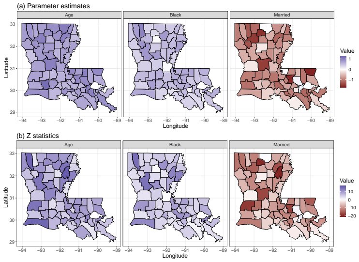
- A natural public-health product would be significance maps of racial disparities in survival, where the paper's Z-statistic maps already hint at geographic variation.
- The graph-distance neighborhood scheme could also be combined with per-covariate bandwidths, allowing some effects to vary globally while others vary locally; the paper lists this direction but does not implement it.
Signed reviews
Editorial analysis
A structured set of objections, weighed in public.
Referee Report
Summary. The paper proposes a geographically weighted Cox regression model for areal survival data. Each observation's contribution to the local partial likelihood at a county s is weighted by an exponential decay of graph distance between the observation's county and s, with the target county and its immediate neighbors receiving weight 1 (Eq. 8). The bandwidth h in the weight function is chosen by a Takeuchi information criterion (Eq. 10). The authors state consistency and asymptotic normality of the estimator in Propositions 1-2 under regularity conditions C1-C2 borrowed from Fan et al. (2006) and Wang and Yao (2006). The method is evaluated in simulations with 1000 replicates under no spatial variation and two spatially varying coefficient mechanisms, and applied to SEER prostate cancer data from Louisiana, yielding county-level estimates and Z statistics for age, race, and marital status at h=1.5.
Significance. If the estimation, bandwidth-selection, and inferential claims are valid, the paper addresses a real practical problem: it enables local hazard-ratio estimation in counties too sparse for separate Cox model fits by borrowing strength from neighboring counties, and the graph-distance weighting avoids the subjective choice of a distance threshold used by great-circle-distance schemes. The simulation study is a genuine strength: 1000 replicates, two spatial structures, four performance measures, and comparisons against local, global, and great-circle-distance weighted fits are reported. The graph-distance estimator performed well at the bandwidths highlighted in the simulations. However, the asymptotic theory is not established in the version under review, and the TIC formula does not match the fitted weighted objective; both issues bear directly on the real-data bandwidth choice and the reported standard errors.
major comments (3)
- [Section 3.4, Conditions C1-C2 and Propositions 1-2] The consistency and asymptotic-normality claims are not supported as stated. The weights in (8) are fixed for a chosen h (h=1.5 in Section 5), whereas Condition C2 refers to Theorem 3.2 of Wang and Yao (2006), a kernel-smoothing result whose weights are required to concentrate as the sample size grows. With a fixed set of 64 counties and n growing within counties, the weighted score equation (3) mixes observations from counties at graph distances 2 and 3 with non-negligible weights exp(-1.5) and exp(-3), so its population limit is a smoothed mixture of the true county-specific coefficient vectors, not beta(s). Consistency of beta-hat(s) for the true local coefficient would require either h_n -> 0, a shrinking-neighborhood condition, or an explicit smoothness assumption that makes the smoothed target equal to beta(s); none of these is stated. For the same reason the sqrt(n) rate with a bias term xi(s) in Proposition 2 is not obtained from the cited conditions. The text says the proofs are in the Supplemental Material, but no supplement is present in the arXiv submission, so the claims cannot be checked. The standard errors and Z statistics in Figure 7 rest on this unverified asymptotic justification.
- [Section 3.3, Eq. (10)] The TIC as written is not the TIC of the fitted weighted partial-likelihood model. The log-likelihood term sums, for each county j, only the observations located at s*_j and uses the unweighted risk-set denominator sum_{k in R(T_i)} exp(Z_k^T beta-hat(s*_j)); no w_i(s*_j) appears. The penalty term, by contrast, uses the weighted observed information (4) but a score K_j computed from the unweighted own-county contributions. In the Takeuchi criterion the information and score matrices must refer to the same fitted objective; here they refer to different objectives. Consequently the quantity minimized in Section 5 and Figure 6, and the claimed performance of the best-TIC bandwidths in Tables 3-4, do not establish that the criterion selects a good bandwidth for the proposed estimator. The authors should derive the TIC from the actual weighted local partial likelihood in (2)-(4), or present and justify a composite-likelihood version with matching I and K matrices.
- [Sections 4.2 and 5, TIC-based bandwidth selection] The simulation evidence for the TIC is reported only through the modal selected bandwidth: Tables 3-4 give performance at the most frequently chosen h, but no distribution of selected bandwidths over the 1000 replicates is given. If the TIC frequently selects a poor bandwidth and the mode is unrepresentative, the claim that the proposed criterion effectively chooses a bias-variance tradeoff is not established. In addition, because the real-data bandwidth selection and the simulation evaluation use the same criterion in (10), the concerns about Eq. (10) in the previous comment directly affect the reported h=1.5 and the corresponding county-level estimates.
minor comments (5)
- [Abstract and Section 3.2] The proposed weight function (8) is deterministic, so the term 'stochastic neighborhood weighting' is potentially misleading; clarify the connection to the stochastic neighborhood autoregressive model of White and Ghosh (2009).
- [Section 4.1] In the sentence defining the censoring mixture, the text says '0.1<60> represents a point mass at 60' following the expression '0.1Uniform(0,60) + 0.9<60>'; the point mass should be 0.9<60>.
- [Section 4] The paper states that the code and documentation are available at GitHub but gives no repository link; please include the URL or remove the sentence.
- [Section 5 and Figure 7] Please report per-county event counts and standard errors in a supplementary table, and identify the four counties with fewer than three observations, to make the real-data results reproducible.
- [Introduction, paragraph 2] The claim that no existing literature studies the Cox model with spatially varying coefficients for geographically distributed survival data should be softened or substantiated with a more systematic literature search, as related geographically weighted survival work may exist.
Circularity Check
No load-bearing circularity: the estimator, TIC, and asymptotic claims are not definitionally tied to the quantities they predict; the only mild self-reference is a simulation truth generated from the same graph distance used by the weights.
-
other
[Section 4.2, simulation scenario (12); weights (8) in Section 3.2]
"for another county l, the parameter vector is the transpose of (0.7, 0.5, −0.8) + 0.12 × (the graph distance between county l and St. Charles − mean of graph distance between all other counties and St. Charles)."
The success of the graph-distance weighted model in this scenario is partly engineered: the true coefficient surface (12) is a linear function of the same graph distance that defines the estimating weights in (8). The estimator is therefore validated against a ground truth that already varies along the exact metric assumed by the method. This does not make the derivation circular — the Cox partial-likelihood estimates are still computed from survival data — but it is a self-referential simulation design rather than an independent test of the graph-distance assumption.
full rationale
The central derivation is self-contained: beta-hat(s) solves the weighted score equation (3) built from the local partial likelihood (2), and no target quantity is inserted into the estimating equation. The TIC in (10) is a standard likelihood-based model selection device, and the real-data bandwidth (h=1.5) is chosen by minimizing that TIC; this is selection on the same data, not a fitted parameter renamed as a prediction. Self-citations (Hu 2017; Hu and Huffer 2019) are used for data, an observed KM pattern, and a threshold-weighting ansatz, but none is load-bearing for the paper's consistency/normality claims; those claims instead import external theorems (Fan et al. 2006; Wang and Yao 2006). The true weakness is not circularity: the graph weights in (8) are fixed rather than shrinking, so Conditions C1-C2 (Section 3.4) are not obviously satisfied, and the proof is relegated to a Supplement absent from the arXiv version. That is a rigor/verifiability gap, not an equation-level circularity. Score 1 reflects the minor self-referential simulation scenario (12), not a reduction of the main result to its inputs.
Assumptions & free parameters
free parameters (3)
- Bandwidth h in the exponential graph-distance weight (Eq. 8) =
1.5 in the Louisiana application; grid 0.5 to 20 in real data and 0.5 to 50 in simulations
- Great-circle-distance threshold dl in comparison weighting schemes (Eq. 6) =
Candidate values 0.5, 1, 1.29, 2; real data uses 1, 1.29, and 2
- Scaling of great-circle distances to a maximum of 11 =
11
assumptions (4)
- ad hoc to paper Regularity conditions C1 and C2 from Fan et al. (2006) and Wang and Yao (2006) hold for the graph-distance weighted estimator.
- domain assumption Graph distance on the county adjacency graph is an appropriate measure of geographic proximity.
- domain assumption The proportional hazards assumption holds locally at each county.
- domain assumption All regression coefficients vary spatially.
Cite this review
Pith. "Pith review of Geographically Weighted Cox Regression for Prostate Cancer Survival Data in Louisiana." pith.science (2026). https://pith.science/paper/3SE6UI3H
@misc{pith2026190809071,
  author       = {Pith},
  title        = {Pith review of: Geographically Weighted Cox Regression for Prostate Cancer Survival Data in Louisiana},
  year         = {2026},
  howpublished = {\url{https://pith.science/paper/3SE6UI3H}},
  note         = {Machine review of arXiv:1908.09071}
}
read the original abstract
The Cox proportional hazard model is one of the most popular tools in analyzing time-to-event data in public health studies. When outcomes observed in clinical data from different regions yield a varying pattern correlated with location, it is often of great interest to investigate spatially varying effects of covariates. In this paper, we propose a geographically weighted Cox regression model for sparse spatial survival data. In addition, a stochastic neighborhood weighting scheme is introduced at the county level. Theoretical properties of the proposed geographically weighted estimators are examined in detail. A model selection scheme based on the Takeuchi's model robust information criteria (TIC) is discussed. Extensive simulation studies are carried out to examine the empirical performance of the proposed methods. We further apply the proposed methodology to analyze real data on prostate cancer from the Surveillance, Epidemiology, and End Results cancer registry for the state of Louisiana.
Figures


Figures from the paper (4 more)


Reference graph
Works this paper leans on
-
[1]
Akaike, H. (1973). Information theory and an extension of the maximum likelihood principle. In B. N. Petrov and F. Csaki (Eds.), Second International Symposium on Information Theory , pp.\ 267--281. Akad\' e miai Kiado
work page 1973
-
[2]
Banerjee, S., B. P. Carlin, and A. E. Gelfand (2014). Hierarchical Modeling and Analysis for Spatial Data . CRC press
work page 2014
-
[3]
Banerjee, S. and D. K. Dey (2005). Semiparametric proportional odds models for spatially correlated survival data. Lifetime Data Analysis\/ 11\/ (2), 175--191
work page 2005
-
[4]
Banerjee, S., M. M. Wall, and B. P. Carlin (2003). Frailty modeling for spatially correlated survival data, with application to infant mortality in M innesota. Biostatistics\/ 4\/ (1), 123--142
work page 2003
-
[5]
Bhattacharyya, S. and P. J. Bickel (2014). Community detection in networks using graph distance. arXiv preprint arXiv:1401.3915\/
work page Pith review arXiv 2014
-
[6]
Brunsdon, C., A. S. Fotheringham, and M. E. Charlton (1996). Geographically weighted regression: a method for exploring spatial nonstationarity. Geographical Analysis\/ 28\/ (4), 281--298
work page 1996
-
[7]
Brunsdon, C., S. Fotheringham, and M. Charlton (1998). Geographically weighted regression-modelling spatial non-stationarity. Journal of the Royal Statistical Society: Series D (The Statistician)\/ 47\/ (3), 431--443
work page 1998
-
[8]
Cox, D. R. (1972). Regression models and life-tables. Journal of the Royal Statistical Society. Series B (Methodological)\/ 34\/ (2), 187--220
work page 1972
Show all 34 references
-
[9]
Cox, D. R. (1975). Partial likelihood. Biometrika\/ 62\/ (2), 269--276
1975
-
[10]
Fan, J., H. Lin, Y. Zhou, et al. (2006). Local partial-likelihood estimation for lifetime data. The Annals of Statistics\/ 34\/ (1), 290--325
2006
-
[11]
Fleming, T. R. and D. P. Harrington (1991). Counting Processes and Survival Analysis . New York: Wiley
1991
-
[12]
Fotheringham, A. S., W. Yang, and W. Kang (2017). Multiscale geographically weighted regression (mgwr) . Annals of the American Association of Geographers\/ 107\/ (6), 1247--1265
2017
-
[13]
E., H.-J
Gelfand, A. E., H.-J. Kim, C. Sirmans, and S. Banerjee (2003). Spatial modeling with spatially varying coefficient processes. Journal of the American Statistical Association\/ 98\/ (462), 387--396
2003
-
[14]
Grambsch, P. M. and T. M. Therneau (1994). Proportional hazards tests and diagnostics based on weighted residuals. Biometrika\/ 81\/ (3), 515--526
1994
-
[15]
Hijmans, R. J. (2017). geosphere : Spherical Trigonometry . R package version 1.5-7
2017
-
[16]
Hu, G. (2017). Spatial Statistics and Its Applications in Biostatistics and Environmental Statistics . Ph.\ D. thesis, The Florida State University
2017
-
[17]
Hu, G. and F. Huffer (2019). Modified K aplan-- M eier estimator and N elson-- A alen estimator with geographical weighting for survival data. Geographical Analysis\/ . Forthcoming
2019
-
[18]
Hanson, and J
Li, L., T. Hanson, and J. Zhang (2015). Spatial extended hazard model with application to prostate cancer survival. Biometrics\/ 71\/ (2), 313--322
2015
-
[19]
Brunsdon, M
Lu, B., C. Brunsdon, M. Charlton, and P. Harris (2019). A response to 'a comment on geographically weighted regression with parameter-specific distance metrics'. International Journal of Geographical Information Science\/ 33\/ (7), 1300--1312
2019
-
[20]
He, and K.-T
Mei, C.-L., S.-Y. He, and K.-T. Fang (2004). A note on the mixed geographically weighted regression model. Journal of Regional Science\/ 44\/ (1), 143--157
2004
-
[21]
Szymanski, J
M \"u ller, W., K. Szymanski, J. Knop, and N. Trinajsti \'c (1987). An algorithm for construction of the molecular distance matrix. Journal of Computational Chemistry\/ 8\/ (2), 170--173
1987
-
[22]
Murakami, D., B. Lu, P. Harris, C. Brunsdon, M. Charlton, T. Nakaya, and D. A. Griffith (2019). The importance of scale in spatially varying coefficient modeling. Annals of the American Association of Geographers\/ 109\/ (1), 50--70
2019
-
[23]
Nakaya, T., A. S. Fotheringham, C. Brunsdon, and M. Charlton (2005). Geographically weighted P oisson regression for disease association mapping. Statistics in Medicine\/ 24\/ (17), 2695--2717
2005
-
[24]
Onicescu, G. and A. B. Lawson (2018). Bayesian cure-rate survival model with spatially structured censoring. Spatial Statistics\/ 28 , 352--364
2018
-
[25]
Oshan, T., L. J. Wolf, A. S. Fotheringham, W. Kang, Z. Li, and H. Yu (2019). A comment on geographically weighted regression with parameter-specific distance metrics. International Journal of Geographical Information Science\/ 33\/ (7), 1289--1299
2019
-
[26]
Oshan, T. M., Z. Li, W. Kang, L. J. Wolf, and A. S. Fotheringham (2019). mgwr : A P ython implementation of multiscale geographically weighted regression for investigating process spatial heterogeneity and scale. ISPRS International Journal of Geo-Information\/ 8\/ (6), 269
2019
-
[27]
Takeuchi, K. (1976). The distribution of information statistic and the criterion of the adequacy of a model. Suri-Kagaku (Mathematical Sciences)\/ 3 , 12--18. (in Japanese)
1976
-
[28]
Therneau, T. M. (2017). A Package for Survival Analysis in S . version 2.41-3
2017
-
[29]
Tobler, W. R. (1970). A computer movie simulating urban growth in the D etroit region. Economic Geography\/ 46 , 234--240
1970
-
[30]
Verweij, P. J. and H. C. van Houwelingen (1995). Time-dependent effects of fixed covariates in C ox regression. Biometrics\/ 51\/ (4), 1550--1556
1995
-
[31]
Wang, Q. and L. Yao (2006). Estimation in varying-coefficient proportional hazard regression model. Metrika\/ 64\/ (3), 271--288
2006
-
[32]
White, G. and S. K. Ghosh (2009). A stochastic neighborhood conditional autoregressive model for spatial data. Computational Statistics & Data Analysis\/ 53\/ (8), 3033--3046
2009
-
[33]
Yu, H., A. S. Fotheringham, Z. Li, T. Oshan, W. Kang, and L. J. Wolf (2019). Inference in multiscale geographically weighted regression. Geographical Analysis\/ . Forthcoming
2019
-
[34]
Zhang, J. and A. B. Lawson (2011). Bayesian parametric accelerated failure time spatial model and its application to prostate cancer. Journal of Applied Statistics\/ 38\/ (3), 591--603
2011
Reviewed August 14, 2026 · model on record in the stance chip above.
Discussion (0). Continue with ORCID to comment.