Web-enabled Intelligent System for Continuous Sensor Data Processing and Visualization

Felix G. Hamza-Lup; Ionut E. Iacob; Sushmita Khan

REVIEW 4 major objections 7 minor 23 references

Web-enabled Intelligent System for Continuous Sensor Data Processing and Visualization

T0 review · 4 major / 7 minor · reviewed 2026-08-14 · deepseek-v4-flash

Challenge this review Re-run · record.json Download PDF Read on arXiv ↗ Review JSON

Pith's one-line read Sparse fixed sensors can be turned into a continuous 3D temperature or nitrogen map of an entire monitored room or waterbed, in near real time, by solving the Laplace equation with finite differences and then fitting a neural network to…

desk verdict A clearly described prototype that combines finite differences with ANN smoothing for 3D sensor data visualization, but the absence of real-data validation leaves the physical accuracy claims unsubstantiated. read the letter →

arxiv 1908.09089 v1 pith:RSZKOGFU submitted 2019-08-24 eess.SP cs.HC

Felix G. Hamza-Lup , Ionut E. Iacob , Sushmita Khan This is my paper · ORCID

classification eess.SPcs.HC

keywords sensordatavisualizationX3Dfinitedifferencemethodneuralnetworkapproximationthermalmonitoringnitrogencycleaquaponicsweb-based3Dheatmaps

verification ladder T0 review T1 audit T2 compute T3 formal

The pith

A machine-rendered reading of the paper's core claim, the machinery that carries it, and where it could break.

The reading

Monitoring a room or an aquaponics tank usually means looking at a handful of point readings. This paper claims that those sparse readings are enough to reconstruct a continuous, interactive 3D picture of the whole interior: temperatures in a building or nitrogen-compound concentrations in a waterbed. The recipe is to interpolate the sensor values on the boundaries, solve the steady-state heat (diffusion) equation on a coarse grid using finite differences, and then train a single-hidden-layer neural network to act as a smooth, everywhere-defined stand-in for the field. The authors report that the finite-difference stage takes about 112 ms per update on a standard laptop, and that with a 500 ms data-fetch buffer the pipeline can sustain more than 25 interactive frames per second of X3D visualization in a web browser. If the approach holds, building managers and aquaponics operators would gain a live spatial view of heat or nitrogen distribution from inexpensive static sensors, along with a compact analytic model that supports zooming and anomaly checks.

What carries the argument

The load-bearing pair is (i) the Laplace equation with Dirichlet boundary conditions $\Delta u = 0$ on $\Omega=(0,1)^3$, and (ii) the approximation network $u(x,y,z) \approx N(x,y,z) = \sum_{i=1}^{L} Z_i \sigma(W_{1i}x+W_{2i}y+W_{3i}z+b_{1i}) + b_2$. The Laplace equation is the physical prior: with the volume treated as homogeneous and at steady state, boundary values determine the interior, which justifies reconstructing the field from a few boundary sensors. Finite differences convert that equation into a linear system solved once on an intermediate grid ($8 \times 8 \times 8$); the neural network then replaces the discrete solution with a smooth analytic formula, a step the paper justifies by the universal approximation theorem. This combination is what carries the system's claimed capabilities: zooming to arbitrary resolution, evaluating the field at any point, and flagging anomalies from short-term estimates.

What would settle it

Place a heat source or an active nitrogen-producing biofilter inside the monitored volume and record the resulting field with a dense grid of reference sensors; if the sparse-boundary reconstruction fails to reproduce the interior maximum or systematically misestimates gradients, the homogeneous steady-state Laplace assumption is experimentally falsified.

Watch

Extended reading notes

Core claim

On its own terms, the paper's contribution is a 'data stuffing' pipeline that turns sparse sensor readings into a full-volume scalar field. Given the eight corner values of a cube (or eight corners plus six face-center values), the system constructs Dirichlet boundary conditions by linear interpolation on each face, solves the homogeneous Laplace equation on a regular $8 \times 8 \times 8$ grid with finite differences, and then fits a network $N(x,y,z)$ with one hidden layer and sigmoid activations so that $u(x,y,z) \approx N(x,y,z)$ throughout the domain. The resulting analytic approximation is evaluated on a finer $16 \times 16 \times 16$ grid and rendered as semitransparent X3D box primitives in a web browser. The same pipeline is demonstrated with predefined values for nitrogen compounds in an aquaponics waterbed, and the authors frame this as an extension of their earlier linear-interpolation thermal maps to a physically motivated diffusion model.

Load-bearing premise

The entire reconstruction treats the monitored volume as a homogeneous cube in steady state, so a handful of interpolated boundary readings are assumed to determine the whole interior through the Laplace equation.

Editorial extensions

If this is right

A room equipped with 8 to 14 fixed sensors could display a live 3D temperature map in a browser at interactive frame rates, with the finite-difference update costing about 112 ms per reading.
The neural-network output is an analytic function of position, so the visualization can be refined or zoomed without rerunning the numerical solver, and the same function can generate arrays at any resolution.
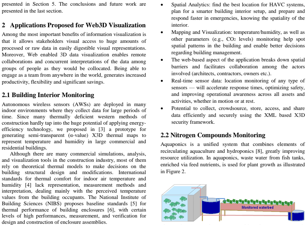
The same computational pipeline transfers from room temperature to nitrogen-compound concentration in an aquaponics waterbed, as long as the scalar field obeys the same steady-state diffusion model.
Because the analytic formula can be evaluated quickly, the system can generate short-term lookahead estimates from recent sensor history, which the authors propose as a basis for detecting sudden events such as fires, waterbed failures, or sensor faults.
The pipeline targets web-standard X3D, so the resulting 3D scenes are shareable across collaborators without specialized visualization software.

Reading between the lines

Editorial extensions of the paper, not claims the author makes directly.

Relaxing the homogeneous steady-state assumption would not break the machinery: replacing the constant coefficient with a spatially varying diffusivity, or adding a source term for biological nitrogen flux, would keep the FD+ANN pipeline intact while making the reconstructions valid for real rooms with windows and HVAC flow or for active biofilters.
The analytical representation also gives closed-form gradients, so the system could locate hot spots, insulation gaps, or stagnant zones by thresholding $\nabla u$—an extension the paper does not pursue but that follows immediately from its model.
The paper's performance numbers imply a natural two-tier update policy: stream the cheap FD refresh for live monitoring and reserve the 64-second ANN fit for historical or zoomed views; a drift-triggered refit rule is a testable next step.
The anomaly-detection claim inherits the model's weakness: if the real field departs from Laplace, the detector will flag model error as an event. Calibrating the system against dense reference measurements would separate genuine anomalies from reconstruction artifacts.

Share X Bluesky LinkedIn Reddit HN

Signed reviews

No signed human review yet.

Editorial analysis

A structured set of objections, weighed in public.

Desk editor's note, referee report, and a circularity audit.

Desk Editor's Note

read the letter

Read the paper. The useful bit is the pipeline: sparse sensor readings on a cube are interpolated to boundary values, a Laplace equation is solved via finite differences, and a single-hidden-layer ANN is fit to the FD grid to produce a compact analytical approximation. That ANN step is new relative to the authors' earlier linear-interpolation thermal maps, and the aquaponics application is a new domain. The math is standard and correctly applied, the recursive cube decomposition is a nice touch, and the authors are upfront about the ANN training cost (64s) and suggest running it only for zoom/playback. Credit where due: this is a real prototype, not just a sketch.

The main soft spot is validation. Everything is synthetic—Table 1 gives eight corner temperatures, and all results are for that snapshot. There is no comparison against measured data, thermal imaging, or any ground truth in a real room or waterbed. Worse, the ANN is trained on the FD output and then used to 'refine' that same FD output, so the accuracy demonstrated is interpolation of an interpolation. That is fine for smoothing, but it does not show the maps represent the physical environment. The paper itself concedes (Section 3.2) that windows or shared walls introduce significant nonlinearity, yet the model still assumes a homogeneous steady-state cube. For aquaponics, the nitrogen cycle has volumetric sources and sinks, so the Laplace equation is even more obviously an idealization. I am not saying the model is useless in its niche; I am saying the paper never gives a reason to trust it.

The near real-time claim also needs care. Step 3 takes 64 seconds, so they push it offline. Steps 1+2 take 112ms, giving roughly a 9 Hz data refresh rate, not 25+ fps. The 500ms buffer and 25+ fps appear to refer to rendering interactivity, not data update rate, but the paper does not clearly separate the two. Minor clarity issue, resolvable on a close read.

For reproducibility, the ANN details are thin: no hidden neuron count L, no training algorithm, no learning rate, no epochs, no final error measure. A reader would have to guess.

Overall: the pipeline is plausible and the implementation is real, but the physical-accuracy claims are unsubstantiated. I would not cite this as evidence for the reliability of such maps, but I would send it to peer review—the core idea is clear, and a serious referee could push the authors to add real data or significantly soften their conclusions. As is, it is a conditional accept at best, and for a short Web3D paper that may be enough.

Referee Report

4 major / 7 minor

Summary. The paper proposes a prototype system for continuous sensor data processing and web-based 3D visualization using the X3D standard, targeting two applications: building thermal monitoring and nitrogen-cycle monitoring in aquaponics waterbeds. The processing pipeline consists of three steps: (i) sparse sensor readings are used to construct boundary values via linear or 2D diffusion interpolation, (ii) the Laplace equation is solved on a regular 3D grid using a finite differences (FD) method, and (iii) a neural network (ANN) is trained on the FD output to produce an analytical approximation of the field, enabling arbitrary-resolution evaluation and interactive 'zooming'. The paper reports a simulated experiment on a unit cube with synthetic sensor values (Table 1), latency measurements for data communication, and X3D visualization examples.

Significance. The central idea—using a neural network as a compact, analytical surrogate for a numerical PDE solution—is conceptually attractive and could enable interactive exploration of sparse sensor data in web-based 3D interfaces. The recursive geometry decomposition and the X3D visualization pipeline are also useful starting points. However, the current contribution is severely limited by the lack of any validation: the sensor inputs are synthetic, the ANN is trained on and evaluated against the same FD output, and the physical model (steady-state Laplace) is never tested against real measurements or an analytical ground truth. If the framework were validated, it could be a valuable tool for building management and aquaponics, but as presented the results only demonstrate that the software pipeline is executable.

major comments (4)

[Section 5.2, Table 1] The experimental evaluation uses entirely synthetic sensor values (locations and 19–27 degree-like numbers) with no stated source, calibration, or ground truth. The paper claims these are 'sensor reading values' but provides no evidence that they represent real measurements from either a building or an aquaponics system. Since the central claim is that the visualization represents physical temperature or nitrogen distributions, the absence of any validation against a known solution (e.g., an analytical harmonic function) or dense reference measurements makes the results uninterpretable as a test of the system's predictive ability.
[Section 5.2, step 3, Figure 7] The ANN is trained on the set S, which is itself the output of the FD solver on the 8×8×8 grid, and is then used to produce a refined 16×16×16 grid and to 'smooth' the FD approximation. Because S is generated entirely by the FD model, the ANN can only learn to reproduce that model's behavior; any bias or error in the FD solution (including those from the boundary interpolation and the Laplace assumption) is propagated unchanged. There is no error metric comparing the ANN output to independent data, so the refinement step demonstrates interpolation of the training set, not improved physical accuracy or a validation of the underlying model.
[Section 5.1, Eq. (2); Section 3.2] The load-bearing modeling assumption is that each monitored volume is a homogeneous cube in steady state, so the field satisfies the Laplace equation with Dirichlet boundary conditions interpolated from sparse sensor readings. The paper itself acknowledges in Section 3.2 that windows, shared walls, and external sun/shade introduce significant nonlinearity, and for the aquaponics scenario nitrogen has volumetric sources and sinks (fish excretion, nitrification, plant uptake) that the Laplace equation does not represent. This assumption is never tested against real measurements. If the assumption is violated, the reconstructed field is an idealized harmonic interpolation, not a representation of the physical environment, which would invalidate the core visualization claim.
[Section 4.2] The 'near real-time, continuous' claim is supported only by separately measured component latencies: 80ms transmission, 95ms reading, 112ms processing (steps 1–2), and a 500ms data-fetch buffer. However, step 3 (ANN training) takes 64s on the reported platform. The paper states that step 3 need not be performed for every reading, but then the continuously displayed data are the coarse FD grid, not the 'refined' analytical representation that motivates the ANN. No end-to-end measurement of the complete pipeline (sensor acquisition through X3D rendering) under continuous operation is provided, so the performance claim is not substantiated.

minor comments (7)

[Section 4] The paragraph after Section 3.2 contains an incomplete sentence: 'Section 4 presents the sensor system and data collection process. general description of the whole process, as well as the details of the underlying model we propose. The general description of the whole framework and the underlying model we propose, and our experimental results are presented in Section 5.' This appears to be a copy-paste artifact and should be rewritten.
[Section 5.2] In the definition of S2, the last element is written as 'u(1, 0.5, 0.5, 0.5)' with four coordinates; it should be 'u(1, 0.5, 0.5)' to match the (x,y,z) domain.
[Section 5.2, Eq. (1)] The number of hidden neurons L in the ANN is never specified in the experiments. Please report the chosen value, the activation function (sigmoid is implied), the training algorithm, and the number of epochs, since these affect the reproduction of the results.
[Table 1] The sensor values are given without units or a statement about whether they are calibrated readings or arbitrary simulation values. Please clarify what physical quantity these numbers represent (e.g., degrees Celsius or a normalized index).
[Figures 6 and 7] The figures lack sufficient caption detail: there is no color scale, no axis labels, and no explicit indication of which data set (S1 or S2, linear vs. diffusion boundary interpolation) is being shown. Please add captions that allow the reader to interpret the visualizations.
[Section 1] The introduction refers to 'α-values' for transparency but never defines α; please define the transparency parameter when it is first used.
[Section 4.1] The sentence 'Going inwards we further divide the cube in sub-cubes' is a sentence fragment; consider revising to 'Going inwards, we further divide the cube into sub-cubes...'

Circularity Check

0 steps flagged · score 0.0 of 10

No significant circularity; the FD-to-ANN pipeline is a transparent surrogate, with physical-fidelity limitations outside the scope of circularity analysis.

full rationale

The derivation chain is transparent and self-consistent. Section 5.1 posits a steady-state Laplace equation (Eq. 2) with Dirichlet boundary values obtained by interpolating sparse sensor readings; Section 5.2 produces a finite-difference solution S on an 8x8x8 grid and then explicitly trains the ANN (Eq. 1) on S to obtain a smooth analytical surrogate. None of these steps defines an output in terms of the paper's conclusion, and no result is imported from the authors' prior work to force the choice: references [3] and [7] are contextual descriptions of earlier prototypes, not load-bearing. The ANN fit to the FD grid means the refined 16x16x16 visualization is an interpolation of the FD solution rather than independent evidence about physical temperatures, but the paper presents this as 'data stuffing' and 'smoothing' rather than as empirical validation. The conceded limitation in Section 3.2 that a window or shared wall 'would introduce significant non-linearity in the model' is a physical-fidelity concern, not a circularity. Therefore no circular step is exhibited.

Assumptions & free parameters 3 free parameters · 6 assumptions · 0 invented entities

The central claim rests on the steady-state Laplace model, the sufficiency of sparse boundary interpolation, and the ANN's ability to fit the FD solution. No new physical entity is introduced. The main free parameters are the ANN hidden-layer count, grid resolutions, and the buffer size behind the real-time claim.

free parameters (3)

Number of hidden neurons L in the ANN
Introduced in Eq. (1); the paper states that L can only be determined by practical trials and does not report the value used for the experiments in Figures 6 and 7.
Grid resolutions = 8x8 face grid, 6x6x6 interior grid, 16x16x16 refinement
Chosen by hand in Section 5.2; these choices affect FD accuracy and ANN training cost, with no grid-convergence study.
Data-fetch buffer size = 500 ms
Introduced in Section 4.2 to hide packet jitter; this value directly supports the claimed 25+ FPS continuous display.

assumptions (6)

domain assumption Each monitored volume is a homogeneous cube and can be scaled from a rectangular parallelepiped without loss of generality.
Invoked in Sections 4.1 and 5.1; real rooms and waterbeds contain windows, convection, and biological activity.
domain assumption The scalar field has reached steady state, so the heat equation reduces to the Laplace equation.
Section 5.1 explicitly says 'for simplicity' steady state; transient effects such as HVAC cycles and feeding schedules are excluded.
domain assumption Boundary values on each face can be interpolated from sparse sensor points using linear interpolation or a 2D FD solve.
Section 5.2 step 1; no evidence is given that 8 or 14 sensors determine the full boundary conditions.
standard math A feedforward neural network with one hidden layer can approximate the FD solution to arbitrary precision.
Universal approximation theorem [14,15] cited in Section 3.1; standard, but it does not specify the required L or training data.
standard math Finite-difference discretization of the Laplace equation yields a sufficiently accurate numerical solution on the chosen grid.
Used in Section 5.2; no grid-convergence or error analysis is provided.
ad hoc to paper The sensor values in Table 1 are representative of real building or aquaponics readings.
Section 5.2 uses these values only for simulation; no real deployment data are collected.

how reviews work

0 comments

Cite this review

Pith. "Pith review of Web-enabled Intelligent System for Continuous Sensor Data Processing and Visualization." pith.science (2026). https://pith.science/paper/RSZKOGFU

@misc{pith2026190809089,
  author       = {Pith},
  title        = {Pith review of: Web-enabled Intelligent System for Continuous Sensor Data Processing and Visualization},
  year         = {2026},
  howpublished = {\url{https://pith.science/paper/RSZKOGFU}},
  note         = {Machine review of arXiv:1908.09089}
}

read the original abstract

A large number of sensors deployed in recent years in various setups and their data is readily available in dedicated databases or in the cloud. Of particular interest is real-time data processing and 3D visualization in web-based user interfaces that facilitate spatial information understanding and sharing, hence helping the decision making process for all the parties involved. In this research, we provide a prototype system for near real-time, continuous X3D-based visualization of processed sensor data for two significant applications: thermal monitoring for residential/commercial buildings and nitrogen cycle monitoring in water beds for aquaponics systems. As sensors are sparsely placed, in each application, where they collect data for large periods (of up to one year), we employ a Finite Differences Method and a Neural Networks model to approximate data distribution in the entire volume.

Figures

Figures reproduced from arXiv: 1908.09089 by the authors.

**Figure 1.** (a) 2D IR thermal image (b) X3D thermal maps from simulated sensor data. Among the advantages of the proposed system are:  Spatial Analytics: find the best location for HAVC systems, plan for a smarter building interior setup, and prepare and respond faster in emergencies, knowing the spatiality of the interior.  Mapping and Visualization: temperature/humidity, as well as other parameters (e.g., CO2 levels) monito… view at source ↗

**Figure 3.** Artificial Neural Network (ANN) model An Artificial Neural Network (ANN) model with one hidden layer and L hidden neurons is represented in [PITH_FULL_IMAGE:figures/full_fig_p003_3.png] view at source ↗

Figures from the paper (1 more)

**Figure 8.** Figure 8: X3D based visualization of diffused temperature maps. For the aquaponics waterbed we implemented a basic setup using predefined values as illustrated in [PITH_FULL_IMAGE:figures/full_fig_p006_8.png]

Discussion (0). Continue with ORCID to comment.

Reference graph

Works this paper leans on

23 extracted references · 22 canonical work pages

[1]

F.; Brutzman, D.; Steed, A.; Behr, J

Polys, N. F.; Brutzman, D.; Steed, A.; Behr, J. Future Standards for Immersive VR: Report on the IEEE Virtual Reality 2007 Workshop. IEEE Computer Graphics and Applic ations, 28 (2):94 -99, 2008, Extensible 3D (X3D), Web3D Consortium. Available online: www.web3d.org (accessed on 09. 09. 2018)

work page 2007
[2]

Adaptive Group- based Zero Knowledge Proof -Authentication Protocol (AGZKP-AP) in Vehicular Ad Hoc Networks,

A. A. Rashid, R. N. Mahapatra, and F. G. Hamza-Lup (2019) “Adaptive Group- based Zero Knowledge Proof -Authentication Protocol (AGZKP-AP) in Vehicular Ad Hoc Networks,” IEEE Transactions of Intelligent Transportation Systems

work page 2019
[3]

G.; Borza, P

Hamza-Lup, F. G.; Borza, P. N.; Dragut, D.; Maghiar , M. X3D Sensor -based Thermal Maps for Residential and Commercial Buildings, Web3D, 2015, Heraklion, Crete, Greece, June 18-21

work page 2015
[4]

Nicol, F., Humphreys, M., Sykes, O., and Roaf, S. (1995). Standards for thermal comfort. TJ Press Ltd., UK

work page 1995
[5]

National Performance Based Design Guide

NIBS (201 9). National Performance Based Design Guide. Building Envelope Design Guide. Available online at: http://www.wbdg.org/guides - specifications/building-envelope-design-guide. Retrieved Mar.6, 2019

work page 2019
[6]

Available online at: https://www.ashrae.org/technical- resources/standards-and-guidelines

Ashrae, 2019. Available online at: https://www.ashrae.org/technical- resources/standards-and-guidelines

work page 2019
[7]

G.; Maghiar, M

Hamza-Lup, F. G.; Maghiar, M. Web3D Graphics enabled through Sensor Networks for Cost -Effective Assessment and Management of Energy Efficiency in Buildings, Graphical Models Journal, Elsevier, 2016

work page 2016
[8]

USDA 2019, https://www.nal.usda.gov/afsic/aquaponics

work page 2019

Show all 23 references

[9]

V., Treadwell, D

Tyson, R. V., Treadwell, D. D., & Simonne, E. H. (2011). Opportunities and Challenges to Sustainability in Aquaponic Systems, HortTechnology hortte, 21(1), 6 -13. Retrieved Mar 13, 2019, from https://journals.ashs.org/view/journals/horttech/21/1/article -p6.xml

2011
[10]

Annual Review of Environment and Resources

Klinger, Dane, Naylor, Rosamond (2012) Searching for Solutions in Aquaculture: Charting a Sustainable Course . Annual Review of Environment and Resources. https://doi.org/10.1146/annurev-environ-021111-161531

2012 doi
[11]

Somerville, M

C. Somerville, M. Cohen, E. Pantanella, A. Stankus, A. Lovatelli Small -scale aquaponic food production: integrated fish and plant farming U. FAO (Ed.), FAO Fisheries and Aquaculture Technical Paper (2014), pp. 1 -262 Rome, Italy

2014
[12]

Dietary protein source or energy levels have no major impact on growth performance, nutrient utilisation or flesh fatty acids composition of market sized Senegalese sole

Valente, L.M.P., Linares, F., Villanueva, J.L.R., Silva, J.M.G., Espe, M., Escorcio, C., Pires, M.A., Saavedra, M.J., Borges, P., Medale, F., Alvarez - Blazquez, B., Peleteiro, J.B., (2011). Dietary protein source or energy levels have no major impact on growth performance, nu...

2011
[13]

Hargreaves J. A. , 1998 Nitrogen biogeochemistry of aquaculture ponds. Aquaculture 166:181-212

1998
[14]

Approximations by superpositions of sigmoidal functions

Cybenko, G. (1989) "Approximations by superpositions of sigmoidal functions", Mathematics of Control, Signals, and Systems, 2(4), 303 –314

1989
[15]

Approximation Capabilities of Multilayer Feedforward Networks

Kurt Hornik (1991) "Approximation Capabilities of Multilayer Feedforward Networks", Neural Networks, 4(2), 251–257

1991
[16]

Multilayer feedforward networks are universal approximators

Hornik, K., Stinchcombe, M., White, H., (1989) “Multilayer feedforward networks are universal approximators”, Neural Networks, 2(5), 359 -366

1989
[17]

Artificial neural networks for solving ordinary and partial differential equations,

I. E. Lagaris, A. Likas and D. I. Fotiadis, "Artificial neural networks for solving ordinary and partial differential equations," in IEEE Transactions on Neural Networks, vol. 9, no. 5, pp. 987-1000, Sept. 1998

1998
[18]

Overcoming the curse of dimensionality: Solving high -dimensional partial differential equations using dee p learning

Han, Jiequn, Jentzen, Arnulf, et al. “Overcoming the curse of dimensionality: Solving high -dimensional partial differential equations using dee p learning”. arXiv preprint, arXiv:1707.02568, 2017

2017 arXiv
[19]

Chung, D. (2015). Historic Building Façades: Simulation, Testing and Verification for Improved Energy Modeling. Journal of the National Institute of Building Sciences, Feb., (3), No. 1, 16-21

2015
[20]

Multi -column deep neural networks for image classification

Ciresan, Dan; Ueli Meier; Jürgen Schmidhuber (2012). Multi -column deep neural networks for image classification. 2012 IEEE Conference on Computer Vision and Pattern Recognition. pp. 3642–3649

2012
[21]

Sensirion Relative-Humidity Sensor

SENSIRION (2019 ) “Sensirion Relative-Humidity Sensor”. Specifications online at: http://www.sensirion.com/. Accessed March 10, 2019

2019
[22]

Orbisphere (2019) https://www.hach.com/nitrogen-sensors/orbisphere-315xx- nitrogen-sensors/family?productCategoryId=35547372750

2019
[23]

ISENO (2019) https://www.hach.com/hq440d-water-quality-laboratory-ise- ammonia-nh-and-nitrate-no-sup-sup-ion-meter-package-with-isenh3181- iseno3181-ion-selective-electrodes/product?id=7640592116&callback=qs

2019

Pith tools

Reviewed August 14, 2026 · model on record in the stance chip above.

[1] [1]

F.; Brutzman, D.; Steed, A.; Behr, J

Polys, N. F.; Brutzman, D.; Steed, A.; Behr, J. Future Standards for Immersive VR: Report on the IEEE Virtual Reality 2007 Workshop. IEEE Computer Graphics and Applic ations, 28 (2):94 -99, 2008, Extensible 3D (X3D), Web3D Consortium. Available online: www.web3d.org (accessed on 09. 09. 2018)

work page 2007

[2] [2]

Adaptive Group- based Zero Knowledge Proof -Authentication Protocol (AGZKP-AP) in Vehicular Ad Hoc Networks,

A. A. Rashid, R. N. Mahapatra, and F. G. Hamza-Lup (2019) “Adaptive Group- based Zero Knowledge Proof -Authentication Protocol (AGZKP-AP) in Vehicular Ad Hoc Networks,” IEEE Transactions of Intelligent Transportation Systems

work page 2019

[3] [3]

G.; Borza, P

Hamza-Lup, F. G.; Borza, P. N.; Dragut, D.; Maghiar , M. X3D Sensor -based Thermal Maps for Residential and Commercial Buildings, Web3D, 2015, Heraklion, Crete, Greece, June 18-21

work page 2015

[4] [4]

Nicol, F., Humphreys, M., Sykes, O., and Roaf, S. (1995). Standards for thermal comfort. TJ Press Ltd., UK

work page 1995

[5] [5]

National Performance Based Design Guide

NIBS (201 9). National Performance Based Design Guide. Building Envelope Design Guide. Available online at: http://www.wbdg.org/guides - specifications/building-envelope-design-guide. Retrieved Mar.6, 2019

work page 2019

[6] [6]

Available online at: https://www.ashrae.org/technical- resources/standards-and-guidelines

Ashrae, 2019. Available online at: https://www.ashrae.org/technical- resources/standards-and-guidelines

work page 2019

[7] [7]

G.; Maghiar, M

Hamza-Lup, F. G.; Maghiar, M. Web3D Graphics enabled through Sensor Networks for Cost -Effective Assessment and Management of Energy Efficiency in Buildings, Graphical Models Journal, Elsevier, 2016

work page 2016

[8] [8]

USDA 2019, https://www.nal.usda.gov/afsic/aquaponics

work page 2019