REVIEW 3 major objections 5 minor 19 references
Disjunct Support Spike and Slab Priors for Variable Selection in Regression under Quasi-sparseness
T0 review · 3 major / 5 minor · reviewed 2026-08-14 · deepseek-v4-flash
Pith's one-line read Spike-and-slab priors with disjoint supports make Bayes factors grow exponentially, restoring consistent variable selection in quasi-sparse regression.
desk verdict The interval spike prior is a sound idea and the paper is worth engaging, but Theorem 1 proves only exponential growth from below, not the convergence to a constant the text claims. read the letter →
The pith
A machine-rendered reading of the paper's core claim, the machinery that carries it, and where it could break.
The reading
What carries the argument
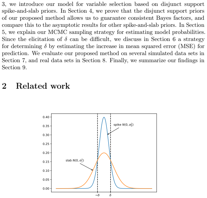
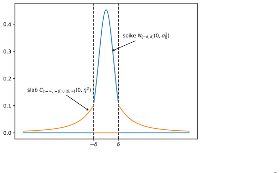
The central object is the disjunct support spike-and-slab prior: a truncated normal spike $\mathcal{N}_{[-\delta,\delta]}(0,\sigma_0^2)$ and a truncated slab (a normal with an inverse-chi-square prior on its variance, giving a Cauchy-like tail) restricted to $|\beta|\ge\delta$, with $\sigma_0$ tuned so the two densities agree at $\pm\delta$. This single construction does two jobs: the threshold $\delta$ encodes an interpretable definition of practical relevance, and the disjoint supports guarantee that any wrong subset assigns zero prior mass to the true coefficients, which is what drives the exponentially growing Bayes factors in Theorem 1; a Gibbs sampler over a latent inclusion vector $z$ then estimates the posterior model probabilities despite the non-conjugate priors.
What would settle it
Simulate a regression where a true coefficient is exactly $\beta_j=\delta$ (or drifts to $\delta$ as $n$ grows) and check whether the log-Bayes-factor ratio in Theorem 1 still diverges to a positive $c$; alternatively, run the Section 6 adaptive $\delta$ procedure on a quasi-sparse design with many coefficients just below $\delta$ and test whether false positives accumulate at large $n$.
Extended reading notes
Core claim
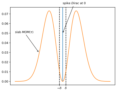
Formally, let $S=\{j:|\beta_{j,t}|>\delta\}$ be the set of practically relevant variables and $S'$ any other set. The paper proves in Theorem 1 that for its disjunct support priors, $(1/n)\log\,[p(y_n|X_n,S)/p(y_n|X_n,S')]\xrightarrow{P} c$ for some $c>0$, so the Bayes factor grows exponentially fast in the sample size. The reason is that the true coefficient vector of a relevant variable lies outside the support of every wrong model's prior; the wrong model's marginal likelihood is then bounded by its constrained maximum likelihood, while the true model's marginal likelihood follows the Laplace approximation, leaving a positive gap in expected log-likelihood. Two companion results sharpen the contrast: Theorem 2 shows that full-support spike-and-slab priors (as in Chipman et al., 2001) yield Bayes factors that are only $O_p(1)$, and Theorem 3 shows that product moment-matching priors (Johnson and Rossell, 2012) make the Bayes factor of the relevant set against the full model converge to $0$ in probability in the quasi-sparse setting, precisely because their spike sits at $\{0\}$ rather than on an interval.
Load-bearing premise
The proof of Theorem 1 assumes the true coefficients never fall exactly on the boundary $\pm\delta$ and that $\delta$ is fixed before the data are collected; the paper's recommended adaptive choice of $\delta$ by expected MSE increase (Section 6) carries no such asymptotic guarantee.
Editorial extensions
If this is right
- Bayes factors under the proposed prior increase at rate $e^{nc}$, so Bayesian hypothesis tests can separate practically relevant covariates from negligible noise once the sample is large enough.
- Full-support spike-and-slab priors give bounded Bayes factors, so their use for formal model testing is questionable even though they are common in practice.
- Product moment-matching priors, while consistent for exact zeros, will asymptotically prefer the model containing every non-zero coefficient, which is the wrong answer in the quasi-sparse setting.
- The latent-variable Gibbs sampler makes the non-conjugate model computationally usable, and the threshold $\delta$ provides an interpretable control on the sparsity-versus-prediction trade-off.
Reading between the lines
- The same disjoint-support construction could plausibly repair Bayes-factor inconsistency in other model classes with quasi-sparse structure, such as generalized linear models or Gaussian graphical models, since the proof only relies on the true parameter falling outside the wrong model's support.
- Because Theorem 1 requires $\delta$ fixed in advance, the adaptive $\delta$ selection of Section 6 is an open theoretical gap; a fully hierarchical prior on $\delta$ might let the data determine practical relevance while preserving consistency.
- The exponential growth rate $c$ suggests a natural sequential-testing rule: stop collecting data once the log Bayes factor crosses a pre-specified threshold, which could give sample-size savings in screening applications.
Signed reviews
Editorial analysis
A structured set of objections, weighed in public.
Referee Report
Summary. The paper proposes a new spike-and-slab prior for linear regression in which the spike and slab have disjoint supports: the spike is a truncated normal on [-δ,δ] and the slab is a scale mixture of truncated normals on the complement. The threshold δ is intended to encode practical relevance, so that coefficients of magnitude smaller than δ are treated as negligible even if nonzero (quasi-sparseness). The central theoretical claim is Theorem 1, which states that for the true model S and any other model S', (1/n) log p(y_n|X_n,S)/p(y_n|X_n,S') converges in probability to a positive constant c, i.e., Bayes factors grow exponentially. Theorem 2 claims that full-support spike-and-slab priors give Bayes factors that are bounded in probability, and Theorem 3 claims that product moment matching priors are unsuitable in the quasi-sparse setting because they eventually select all nonzero coefficients. The paper also gives a Gibbs sampler for posterior model probabilities, a data-driven rule for choosing δ based on estimated MSE increase, and extensive simulations and real-data comparisons.
Significance. If Theorem 1 were fully established as stated, the paper would offer a practical prior class that combines a meaningful practical-significance threshold with provably growing Bayes factors, filling a real gap for quasi-sparse regression. The strengths are a clean prior construction, analytically tractable conditional updates for the Gibbs sampler, and a thorough empirical comparison including high-dimensional settings and several real data sets. Theorems 2 and 3 are useful and mostly straightforward. However, the central theorem is only proved via a lower bound, and the proof's assumptions exclude the high-dimensional and data-driven-δ settings used in the main experiments. These issues make the theoretical contribution weaker than advertised, though the qualitative exponential-growth claim appears plausible and potentially fixable.
major comments (3)
- [Section 4, Theorem 1 and proof after Eq. (3)-(4)] The theorem asserts convergence of (1/n) log BF to a positive constant, but the proof only establishes a lower bound. After the Laplace expansion for the numerator, the denominator is bounded above by the maximized likelihood p(y|X, θhat_{S'}), discarding the integration measure. This gives log BF ≥ n c_Δ - (d+1)/2 log n + O_p(1), hence only liminf (1/n) log BF ≥ c_Δ > 0. No matching upper bound for the Bayes factor (equivalently, no lower bound for the wrong-model marginal likelihood) is supplied. Because the wrong-model support is closed and has boundaries at ±δ, a Laplace-type lower bound is not a cosmetic step: boundary contributions can affect the polynomial-order term. The theorem should either be restated as a liminf/at-least-exponential-growth result, which is sufficient for the paper's qualitative claim, or the missing upper bound should be proved.
- [Section 4, Theorem 1 assumptions vs. Section 7] The proof of Theorem 1 treats the dimension d as fixed: the factor (d+1)/2 log n and the Laplace determinant O_p(1) depend on that. The high-dimensional experiments in Section 7 use d=1000 with n=100 and n=1000, which are outside the theorem's scope; nonetheless Section 7.1 states that these experiments confirm Theorem 1. Additionally, Theorem 1 assumes a fixed δ chosen before data and |β_j,t| ≠ δ, whereas the main 'proposed*' method in Section 6 selects δ from the data via the estimated MSE increase. The paper should explicitly state these scope limitations and either prove an extension for growing d and adaptive δ or soften the claims that the theorem covers the reported experiments.
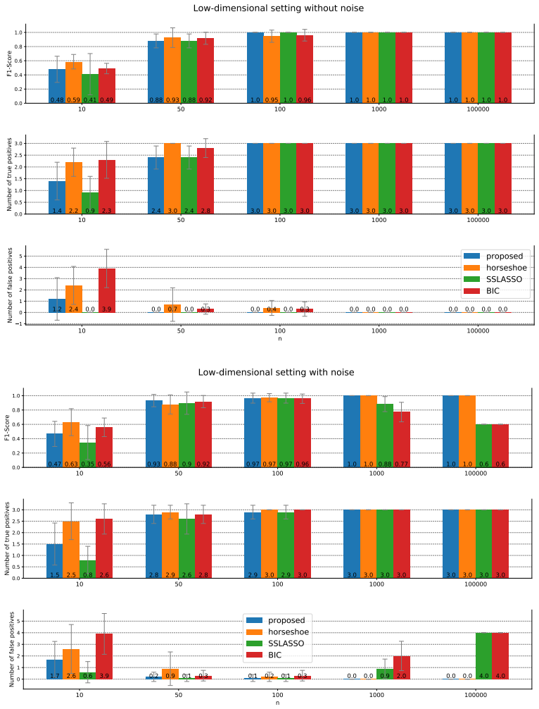
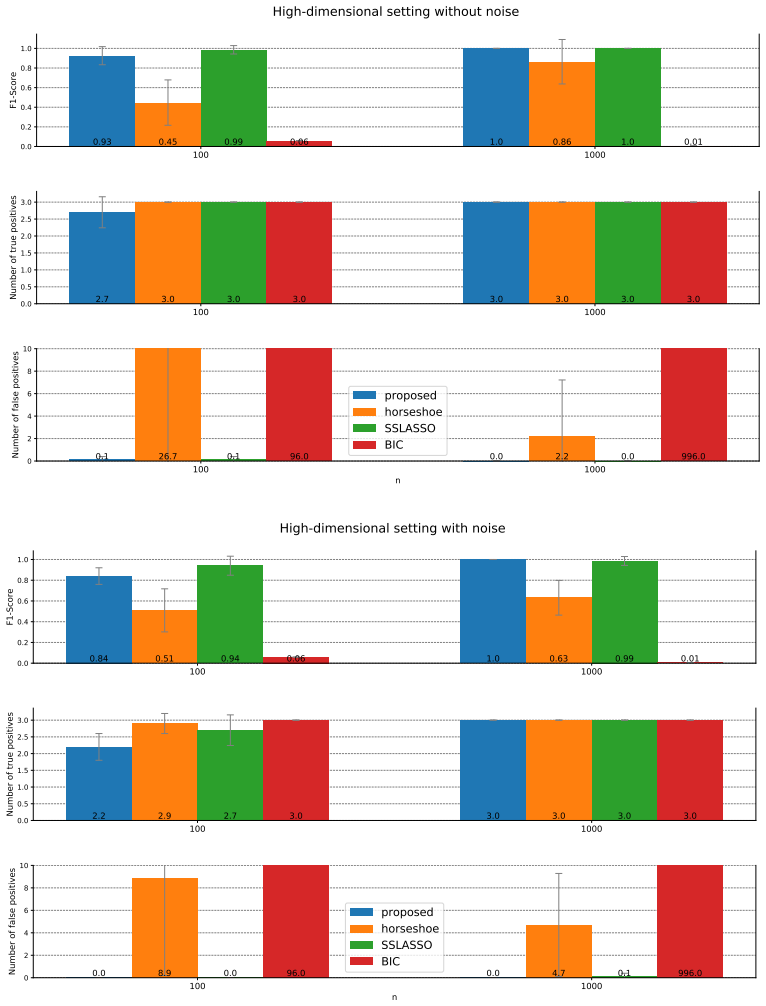
- [Section 7.1 and Table 1] The quantities reported as 'Bayes factors' are not clearly the marginal-likelihood ratios used in Theorem 1. The MCMC procedure in Section 5 estimates posterior model probabilities p(S|y,X); converting these to Bayes factors requires multiplying by the prior odds p(S')/p(S), and the paper does not describe such a conversion. Moreover, the alternative model S' is chosen as the most frequently selected model from the same data, so the comparison is data-dependent rather than a fixed-model Bayes factor. The '∞' entries for cases where the true model is always selected are also not finite Bayes factors and prevent the stated averaging. The authors should clarify the estimand or report Bayes factors against a fixed alternative such as the null or full model.
minor comments (5)
- [Theorem 2 statement] The notation 'P→ Op(1)' is nonstandard; the statement should say that the Bayes factor is bounded in probability, i.e., O_p(1).
- [Section 4, proof of Theorem 1] In the displayed chain near the end of the proof, the notation 'P→' is used on expressions that still contain n; this is informal and should be rewritten as a statement about (1/n) log BF or with explicit o_p(n) error terms.
- [Section 5.4, Eq. (5)] Equation (5) reads 'ι(R,σ1²) ∝ ι(R,σ1²) = (2πσ1²)^{1/2}', which is a tautology in the first part; it should state that ι(R,σ1²) ≈ (2πσ1²)^{1/2} for large σ1² and small δ, as the text intends.
- [Tables 6, 7, and 29] There are typos in the tables: 'Gracia-Donato' should be 'Garcia-Donato', and 'CUNFUC' in Table 29 should be 'CONFUC'. Appendix D also contains 'Tn Table 27' instead of 'In Table 27'.
- [Abstract and Section 7.1] The abstract and Section 7.1 say the experiments 'confirm' Theorem 1 in high-dimensional settings, but Theorem 1 does not apply there; this phrasing should be moderated to say the experiments are suggestive but outside the theorem's assumptions.
Circularity Check
No circularity: the disjunct-support Bayes-factor consistency result is derived from the prior support and standard asymptotics, with no fitted input or self-citation doing load-bearing work.
full rationale
After walking the derivation chain in Sections 3, 4, and 6, I find no step in which a prediction or theorem conclusion is equivalent, by construction or by fitting, to its inputs. Theorem 1 takes the prior with disjunct supports N=[-delta,delta] and R=(-infinity,-delta] union [delta,infinity), defines the true relevant set S={j: |beta_j,t|>delta}, and then proves exponential growth of the Bayes factor. The key mechanism is that beta_t lies outside the support of p(beta|S') for S' != S and inside the support of p(beta|S), so the asymptotic separation c_delta = E_x[g(theta_t)] - E_x[g(theta_S')] > 0 follows from Lemma 1 and p(theta_t|S')=0. No fitted regression quantity enters the theorem. The threshold delta is user-specified, and sigma_0^2 is calibrated by the density-matching equation (1) to make spike and slab densities equal at +/-delta; this is a prior elicitation rule, not a fit to the Bayes factor or to the data. Section 6's data-dependent delta selection is an experimental procedure and is explicitly outside Theorem 1's stated assumptions (the theorem fixes delta and excludes boundary coefficients); that is a scope gap, not circularity. No load-bearing self-citation appears: the external citations to Johnson-Rossell, Kass et al., and Chipman et al. supply standard or independent results, and the authors do not cite their own prior work to justify the central premise. The known weakness of the Theorem 1 proof—it derives only a lower bound on (1/n)log BF, not the claimed convergence—is a correctness/rigor issue, not an instance of the derivation reducing to its own inputs. The central Bayes-factor consistency claim therefore has independent mathematical content relative to the prior specification.
Assumptions & free parameters
free parameters (1)
- threshold δ =
0.5 in BF study; grid {0.8, 0.5, 0.05, 0.01, 0.001, 0.0} in model selection; automatic MSE-based choice in proposed*…
assumptions (4)
- standard math The likelihood and prior satisfy the regularity conditions for the Laplace approximation (Kass et al., 1990), including four-times continuous differentiability of the prior density on an open support.
- domain assumption The covariate distribution is non-degenerate with positive definite covariance; Lemma 1 in Appendix A additionally assumes mean-zero covariates.
- domain assumption The true coefficient vector β_t is not on the boundary of the prior support, i.e. |β_j,t| ≠ δ for all j.
- ad hoc to paper The slab prior is a scale mixture of truncated normals with Inv-χ2(ν1=1, η1^2=100), yielding a truncated Cauchy distribution.
Cite this review
Pith. "Pith review of Disjunct Support Spike and Slab Priors for Variable Selection in Regression under Quasi-sparseness." pith.science (2026). https://pith.science/paper/3MTPHVLH
@misc{pith2026190809112,
  author       = {Pith},
  title        = {Pith review of: Disjunct Support Spike and Slab Priors for Variable Selection in Regression under Quasi-sparseness},
  year         = {2026},
  howpublished = {\url{https://pith.science/paper/3MTPHVLH}},
  note         = {Machine review of arXiv:1908.09112}
}
read the original abstract
Sparseness of the regression coefficient vector is often a desirable property, since, among other benefits, sparseness improves interpretability. In practice, many true regression coefficients might be negligibly small, but non-zero, which we refer to as quasi-sparseness. Spike-and-slab priors as introduced in (Chipman et al., 2001) can be tuned to ignore very small regression coefficients, and, as a consequence provide a trade-off between prediction accuracy and interpretability. However, spike-and-slab priors with full support lead to inconsistent Bayes factors, in the sense that the Bayes factors of any two models are bounded in probability. This is clearly an undesirable property for Bayesian hypotheses testing, where we wish that increasing sample sizes lead to increasing Bayes factors favoring the true model. The moment matching priors as in (Johnson and Rossell, 2012) can resolve this issue, but are unsuitable for the quasi-sparse setting due to their full support outside the exact value 0. As a remedy, we suggest disjunct support spike and slab priors, for which we prove consistent Bayes factors in the quasi-sparse setting, and show experimentally fast growing Bayes factors favoring the true model. Several experiments on simulated and real data confirm the usefulness of our proposed method to identify models with high effect size, while leading to better control over false positives than hard-thresholding.
Figures
Figures from the paper (2 more)
Reference graph
Works this paper leans on
-
[1]
Information theory and an extension of the maximum like- lihood principle
Hirotugu Akaike. Information theory and an extension of the maximum like- lihood principle. In Kitagawa G. Parzen E., Tanabe K., editor,Reprint in Breakthroughs in statistics, 1992, pages 610–624. Springer,
work page 1992
-
[7]
GGCFD3 Average share of expenditures on public investment as fraction of GDP between 1960 and
work page 1960
-
[8]
GOVNOM1 Average share of nominal government spending to nominal GDP between 1960 and
work page 1960
-
[10]
LAAM Dummy for Latin American countries
IPRICE1 Average investment price level between 1960 and 1964 on purchasing power parity basis. LAAM Dummy for Latin American countries. LANDAREA Area in km. LANDLOCK Dummy for landlocked countries. 54 Table 26: Covariates (second part) of SDM data. This table is copied from the description of R package ’BayesVarSel’. LHCPC Log of hydrocarbon deposits in
work page 1960
-
[11]
OIL Dummy for oil-producing country
NEWSTATE National independence. OIL Dummy for oil-producing country. OPENDEC1 Ratio of exports plus imports to GDP, averaged over 1965 to
work page 1965
-
[12]
PI6090 Average inflation rate between 1960 and
work page 1960
-
[13]
SQPI6090 Square of average inflation rate between 1960 and
work page 1960
-
[14]
POP60 Population in 1960 POP6560 Fraction of population older than 65 years in
work page 1960
Show all 19 references
-
[15]
SOCIALIST Dummy for countries under Socialist rule for considerable time during 1950 to
1950
-
[17]
WARTORN Indicator for countries that participated in external war between 1960 and
1960
-
[18]
YRSOPEN Number of years economy has been open between 1950 and
1950
-
[100]
Evaluation results with no noise on regression coefficients
2.4 (0.49) 3.2 (0.4) 48 Table 18: High-dimensional setting,d = 1000 and n∈{ 100, 1000}. Evaluation results with no noise on regression coefficients. Comparison of the proposed method and horseshoe for differentδ. F1-Scores 100 1000 proposed (δ = 0.8) 0.5 (0.0) 0.82 (0.06) propose...
2012
-
[1960]
GEEREC1 Average share public expenditures on education as fraction of GDP between 1960 and
1960
-
[1964]
GOVSH61 Average share government spending to GDP between 1960 and
1960
-
[1965]
DPOP6090 Average growth rate of population between 1960 and
1960
-
[1986]
30 10 50 100 1000 100000 0.0 0.2 0.4 0.6 0.8 1.0F1-Score 0.48 0.88 1.0 1.0 1.00.59 0.93 0.95 1.0 1.00.41 0.88 1.0 1.0 1.00.49 0.92 0.96 1.0 1.0 Low-dimensional setting without noise 10 50 100 1000 100000 0.0 0.5 1.0 1.5 2.0 2.5 3.0Number of true positives1.4 2.4 3.0 3.0 3.02.2...
2012
-
[1990]
ECORG Degree Capitalism index
EAST Dummy for East Asian countries. ECORG Degree Capitalism index. ENGFRAC Fraction of population speaking English. EUROPE Dummy for European economies. FERTLDC1 Fertility in 1960’s. GDE1 Average share public expenditures on defense as fraction of GDP between 1960 and
1960
-
[1995]
TOT1DEC1 Growth of terms of trade in the 1960’s
SPAIN Dummy variable for former Spanish colonies. TOT1DEC1 Growth of terms of trade in the 1960’s. TOTIND Terms of trade ranking TROPICAR Proportion of country’s land area within geographical tropics. TROPPOP Proportion of country’s population living in geographical tropics. W...
1960
-
[2004]
Variables in bold mark the 18 variables that were considered as significant in (Sala-i Martin et al., 2004)
using the BACE method. Variables in bold mark the 18 variables that were considered as significant in (Sala-i Martin et al., 2004). variable δ = 0.5 EAST 0.892 P60 0.485 MALFAL66 0.341 GDPCH60L 0.34 IPRICE1 0.328 TROPICAR 0.285 LIFE060 0.253 CONFUC 0.113 YRSOPEN 0.085 SAFRICA 0...
2004
Reviewed August 14, 2026 · model on record in the stance chip above.
Discussion (0). Continue with ORCID to comment.