REVIEW 3 major objections 7 minor 84 references
Radio Spectroscopic Imaging of a Solar Flare Termination Shock: Split-Band Feature as Evidence for Shock Compression
T0 review · 3 major / 7 minor · reviewed 2026-08-14 · deepseek-v4-flash
Pith's one-line read The split-band radio feature of a solar flare termination shock places the high-frequency lane ~0.8 Mm below the low-frequency lane, supporting an upstream-downstream shock interpretation with an average density compression ratio…
desk verdict Plausible and genuinely new imaging of a termination-shock split band, but the 0.8 Mm spatial offset needs an astrometric control before I would call the scenario confirmed. read the letter →
The pith
A machine-rendered reading of the paper's core claim, the machinery that carries it, and where it could break.
The reading
What carries the argument
The load-bearing object is the split-band feature in the vector radio dynamic spectrum, where the burst group separates into two nearly parallel frequency lanes while remaining resolved into individual stochastic spike bursts, defined as short-lived, narrow-band radio emissions. The key identity that carries the argument is $X = (\nu_{HF}/\nu_{LF})^2$, which converts the observed frequency ratio into a density compression ratio because plasma emission occurs near the local plasma frequency $\nu \propto \sqrt{n_e}$. Complementing this is the precise centroid localization of each spike burst, which allows the paper to measure the vertical offset $\Delta y = y_{HF} - y_{LF}$ at fixed positions along the shock front; this separates the upstream-downstream geometry from variation along the shock front and provides the spatial evidence that the two lanes straddle the shock.
What would settle it
Observe another termination-shock split-band event with the same imaging technique and check whether the high-frequency lane again lies below the low-frequency lane at the same position along the shock front; a reversal of sign, or a large offset that does not track the shock's upstream-downstream orientation, would break the interpretation. A more direct test would be to measure upstream and downstream densities independently, for example from EUV line ratios or from the drift of associated type-III-like bursts, and compare them with $(\nu_{HF}/\nu_{LF})^2$ from simultaneous radio observations.
Extended reading notes
Core claim
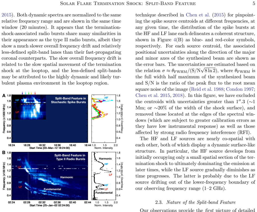
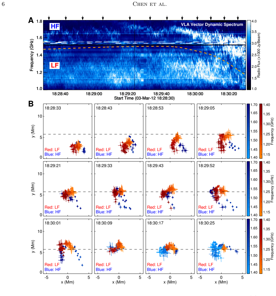
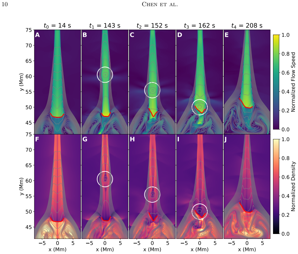
The central claim is that the split-band feature observed in decimetric stochastic spike bursts during the 2012 March 3 flare is produced by plasma radiation from the two sides of a flare termination shock. For each time and position along the shock front, the high-frequency (HF) lane is displaced below the low-frequency (LF) lane by an average of $-0.80\pm 0.02$ Mm, with the distribution of height differences strongly skewed negative; this persistent vertical ordering is what the upstream-downstream scenario predicts, whereas competing explanations would place the two lanes at different positions along the shock front. Under that scenario, the radio frequency $\nu \approx 8980\sqrt{n_e}$ Hz maps directly to electron density, so the density compression ratio across the shock is $X = n_2/n_1 = (\nu_{HF}/\nu_{LF})^2$. The data yield frequency ratios $R_\nu$ between 1.23 and 1.43 and compression ratios $X$ between 1.51 and 2.04, with an average of $X\approx 1.78$, corresponding to a shock Mach number of about 1.6 on average and up to 2.0. The measured spatiotemporal pattern of $X$, including a persistent gradient along the shock front and an asymmetry attributed to impacts of fast plasma blobs, matches the behavior of 2.5D MHD simulations of reconnection outflows hitting flare arcades.
Load-bearing premise
The whole measurement rests on the assumption that both split-band lanes are plasma emission at the same harmonic of the local plasma frequency, so that the frequency ratio directly equals the square root of the density ratio, and that the ~0.8 Mm vertical offset is a true spatial separation rather than a projection or frequency-dependent position artifact.
Editorial extensions
If this is right
- Split-band radio observations can map the density compression ratio along a termination shock front with sub-Mm spatial resolution and sub-second cadence, turning a single shock measurement into a time-resolved two-dimensional diagnostic.
- The inferred average compression $X\approx 1.78$ and Mach number up to 2.0 provide quantitative confirmation of long-standing MHD predictions for flare termination shocks.
- The persistent downward displacement of the high-frequency lane supports the upstream-downstream interpretation of split bands (also called Scenario 1) and suggests that the same interpretation should be applied to, and tested on, split-band type II radio bursts with high-resolution imaging.
- The absence of a matching density-jump signature in EUV images is explained by line-of-sight emission measure, so radio plasma emission can reveal shocks that EUV observations effectively bury.
- The observed asymmetry in compression along the shock front is attributed to impacts of fast plasma blobs or plasmoids, so distorted shock fronts can be recognized and diagnosed from the radio split-band pattern alone.
Reading between the lines
- If the same-harmonic frequency mapping holds across events, the split-band frequency ratio could become a routine remote diagnostic of termination shock Mach number and, indirectly, of the shock's particle-acceleration potential in flares.
- The same centroid-offset method could be applied to high-frequency imaging of type II radio bursts to test whether the upstream-downstream geometry holds at CME-driven coronal shocks, where scattering and projection effects are stronger.
- A testable extension of the MHD comparison is that larger or faster plasmoids should produce larger suppression of the compression ratio on the impacted side of the shock; this prediction could be checked by correlating EUV-detected downflow speeds with the inferred $X(x,t)$ asymmetry in more events.
- If the spectral resolution and cadence are sufficient, one could search for third lanes or harmonic pairs in the spike bursts to directly test the same-harmonic assumption rather than assuming it.
Signed reviews
Editorial analysis
A structured set of objections, weighed in public.
Referee Report
Summary. The paper analyzes the split-band feature observed in decimetric stochastic spike bursts associated with a flare termination shock, using VLA dynamic spectroscopic imaging. The authors find that the high-frequency (HF) lane of the split band is located slightly below the low-frequency (LF) lane, with an average vertical offset of Δy = −0.80 ± 0.02 Mm. They interpret this as evidence for the shock upstream–downstream scenario, in which the HF and LF lanes correspond to plasma emission from the downstream and upstream sides of the shock front, respectively. From the frequency ratio they derive a density compression ratio X = (ν_HF/ν_LF)^2 ≈ 1.78 and a Mach number up to 2.0. They also construct spatially and temporally resolved maps of the compression ratio and compare them with 2.5D MHD simulations, finding qualitative agreement with the effects of plasmoid impacts on the shock front. The paper concludes that the split-band feature provides strong observational evidence for shock compression at a flare termination shock.
Significance. If the central claim holds, this is the first direct, spatially resolved measurement of the upstream–downstream density jump at a flare termination shock, providing quantitative constraints on the shock compression ratio and Mach number that are relevant to particle acceleration and to the interpretation of split-band features in type II radio bursts. The paper is commendable for its careful use of high-cadence VLA spectroscopic imaging, for explicitly considering alternative scenarios (Scenario 1 vs. Scenario 2), and for honestly listing several limitations, including projection effects, the lack of EUV density signatures, and the qualitative nature of the MHD comparison. The quantitative central claim, however, rests on a small spatial offset whose statistical significance is not robust against frequency-dependent astrometric systematics, so the current manuscript is not yet suitable for acceptance.
major comments (3)
- [Section 2.3, Figure 5A] This is a load-bearing issue for the central claim and requires a control-source analysis in the same sub-bands or a quantitative bound on frequency-dependent astrometric errors.
- [Section 2.3 and Section 2.4 (X = R_ν^2)] This is also load-bearing because the main quantitative result is the compression ratio and Mach number.
- [Section 2.4, Figures 6 and 7] The authors should soften the language or add a quantitative metric, and clarify which features of the comparison are considered significant.
minor comments (7)
- [Section 2.3, Figure 5A/B] The current text quotes the mean and standard error but does not give N or the number of independent time–x bins.
- [Section 2.2, centroid uncertainty formula] The formula appears correct for a Gaussian source, but a citation would help readers.
- [Figure 4 caption] Please add a colorbar or explicit frequency labels so that the reader can relate symbol color to frequency.
- [Section 2.4, equations (1)–(3)] Also, the text introduces β before defining it in equation (1); please define β explicitly before or immediately after the equation.
- [Section 2.5, Figure 10] This would help the reader follow the argument about the expected EUV intensity jump.
- [Section 2.2] This is a minor numerical consistency issue.
- [General: data availability] This is increasingly standard for ApJ submissions and would be a useful addition.
Circularity Check
No significant circularity: the split-band offset and frequency ratio are measured quantities, not fitted outputs.
full rationale
The paper's new result is a spatial measurement: the high-frequency split-band lane lies 0.80 ± 0.02 Mm below the low-frequency lane at matched x positions (Section 2.3). This offset is obtained directly from VLA centroid analysis and is not an output of the model or of a fit, so it is independent evidence for the upstream-downstream ordering. The compression ratio X = (ν_HF/ν_LF)^2 is a standard plasma-emission mapping (ν ∝ √n_e) applied to observed frequencies; the paper does not fit X to data and then rename it a prediction. The alternative Scenario 2 is explicitly considered and distinguished using the same spatial data, so the interpretation is not assumed by construction. The termination-shock identity of the source is inherited from Chen et al. (2015), a published, externally reviewable observation by overlapping authors; that cited work is independent support rather than an equation recycled here. The MHD comparison is qualitative and the authors explicitly caution that projection and 2.5D simulation limitations preclude detailed reproduction, so the comparison is not used to force the radio-derived compression values. No load-bearing step reduces by definition to its own input; no fitted parameter is relabeled as a prediction. The main vulnerabilities (per-centroid errors, frequency-dependent astrometric systematics, projection effects) are correctness risks, not circularity.
Assumptions & free parameters
assumptions (4)
- domain assumption Observed radio frequency equals the local plasma frequency (ν ≈ 8980 sqrt(n_e) Hz) at each source
- domain assumption The HF and LF split-band lanes originate from the downstream and upstream sides of the same shock front
- standard math Rankine-Hugoniot jump conditions in simplified limits (perpendicular low-beta, or hydrodynamic high-beta) relate compression to Mach number
- domain assumption The 2.5D resistive MHD simulation (Shen et al. 2018) is a qualitatively valid representation of the termination shock
Cite this review
Pith. "Pith review of Radio Spectroscopic Imaging of a Solar Flare Termination Shock: Split-Band Feature as Evidence for Shock Compression." pith.science (2026). https://pith.science/paper/SWDYJYEI
@misc{pith2026190809146,
  author       = {Pith},
  title        = {Pith review of: Radio Spectroscopic Imaging of a Solar Flare Termination Shock: Split-Band Feature as Evidence for Shock Compression},
  year         = {2026},
  howpublished = {\url{https://pith.science/paper/SWDYJYEI}},
  note         = {Machine review of arXiv:1908.09146}
}
read the original abstract
Solar flare termination shocks have been suggested as one of the promising drivers for particle acceleration in solar flares, yet observational evidence remains rare. By utilizing radio dynamic spectroscopic imaging of decimetric stochastic spike bursts in an eruptive flare, Chen et al. found that the bursts form a dynamic surface-like feature located at the ending points of fast plasma downflows above the looptop, interpreted as a flare termination shock. One piece of observational evidence that strongly supports the termination shock interpretation is the occasional split of the emission band into two finer lanes in frequency, similar to the split-band feature seen in fast-coronal-shock-driven type II radio bursts. Here we perform spatially, spectrally, and temporally resolved analysis of the split-band feature of the flare termination shock event. We find that the ensemble of the radio centroids from the two split-band lanes each outlines a nearly co-spatial surface. The high-frequency lane is located slightly below its low frequency counterpart by ~0.8 Mm, which strongly supports the shock upstream-downstream interpretation. Under this scenario, the density compression ratio across the shock front can be inferred from the frequency split, which implies a shock with a Mach number of up to 2.0. Further, the spatiotemporal evolution of the density compression along the shock front agrees favorably with results from magnetohydrodynamics simulations. We conclude that the detailed variations of the shock compression ratio may be due to the impact of dynamic plasma structures in the reconnection outflows, which results in distortion of the shock front.
Figures


Figures from the paper (7 more)




Reference graph
Works this paper leans on
-
[1]
2004, ApJL, 605, L77 Astropy Collaboration, Robitaille, T
Asai, A., Yokoyama, T., Shimojo, M., & Shibata, K. 2004, ApJL, 605, L77 Astropy Collaboration, Robitaille, T. P., Tollerud, E. J., et al. 2013, A&A, 558, A33 Astropy Collaboration, Price-Whelan, A. M., Sip˝ ocz, B. M., et al. 2018, AJ, 156, 123
2004
-
[2]
2004, ApJ, 615, 526
Aurass, H., & Mann, G. 2004, ApJ, 615, 526
2004
-
[3]
2002, A&A, 384, 273
Aurass, H., Vrˇ snak, B., & Mann, G. 2002, A&A, 384, 273
2002
-
[4]
M., Krucker, S., Glesener, L., & Lin, R
Bain, H. M., Krucker, S., Glesener, L., & Lin, R. P. 2012, ApJ, 750, 44
2012
-
[5]
Bale, S. D., Reiner, M. J., Bougeret, J. L., et al. 1999, Geophys. Res. Lett., 26, 1573
work page 1999
-
[6]
Bastian, T. S. 1994, ApJ, 426, 774
1994
-
[7]
Cairns, I. H., Knock, S. A., Robinson, P. A., & Kuncic, Z. 2003, SSRv, 107, 27
work page 2003
-
[8]
Caspi, A., Krucker, S., & Lin, R. P. 2014, ApJ, 781, 43
work page 2014
Show all 84 references
-
[9]
Caspi, A., & Lin, R. P. 2010, ApJL, 725, L161
2010
-
[10]
S., & Gary, D
Chen, B., Bastian, T. S., & Gary, D. E. 2014, ApJ, 794, 149
2014
-
[11]
S., Shen, C., et al
Chen, B., Bastian, T. S., Shen, C., et al. 2015, Science, 350, 1238
2015
-
[12]
S., White, S
Chen, B., Bastian, T. S., White, S. M., et al. 2013, ApJL, 763, L21
2013
-
[13]
2018, ApJ, 866, 62
Chen, B., Yu, S., Battaglia, M., et al. 2018, ApJ, 866, 62
2018
-
[14]
D., Zhang, J., et al
Cheng, X., Ding, M. D., Zhang, J., et al. 2014, ApJL, 789, L35
2014
-
[15]
D., Liu, Y., & Poomvises, W
Cheng, X., Zhang, J., Ding, M. D., Liu, Y., & Poomvises, W. 2013, ApJ, 763, 43
2013
-
[16]
P., Holman, G
Chrysaphi, N., Kontar, E. P., Holman, G. D., & Temmer, M. 2018, ApJ, 868, 79 Claßen, H. T., & Aurass, H. 2002, A&A, 384, 1098
2018
-
[17]
Condon, J. J. 1997, PASP, 109, 166
1997
-
[18]
2015, ApJ, 812, 52
Du, G., Kong, X., Chen, Y., et al. 2015, ApJ, 812, 52
2015
-
[19]
P., & Kennel, C
Edmiston, J. P., & Kennel, C. F. 1984, Journal of Plasma Physics, 32, 429
1984
-
[20]
D., Nita, G
Fleishman, G. D., Nita, G. M., & Gary, D. E. 2017, ApJ, 845, 135
2017
-
[21]
Forbes, T. G. 1986, ApJ, 305, 553
1986
-
[22]
Forbes, T. G. 1988, SoPh, 117, 97
1988
-
[23]
G., & Malherbe, J
Forbes, T. G., & Malherbe, J. M. 1986, ApJL, 302, L67
1986
-
[24]
E., Dulk, G
Gary, D. E., Dulk, G. A., House, L., et al. 1984, A&A, 134, 222
1984
-
[25]
E., & Yoshimura, K
Plowman, J. E., & Yoshimura, K. 2015, ApJ, 800, 54
2015
-
[26]
2012, ApJ, 753, 28 16 Chen et al
Guo, F., & Giacalone, J. 2012, ApJ, 753, 28 16 Chen et al
2012
-
[27]
2017, ApJL, 846, L12
Guo, L., Li, G., Reeves, K., & Raymond, J. 2017, ApJL, 846, L12
2017
-
[28]
G., & Kontar, E
Hannah, I. G., & Kontar, E. P. 2012, A&A, 539, A146
2012
-
[29]
Young, P. R. 2011, ApJ, 741, 107
2011
-
[30]
A., Gallagher, P
Hayes, L. A., Gallagher, P. T., Dennis, B. R., et al. 2019, ApJ, 875, 33
2019
-
[31]
D., & Pesses, M
Holman, G. D., & Pesses, M. E. 1983, ApJ, 267, 837
1983
-
[32]
2013, ApJL, 776, L11
Imada, S., Aoki, K., Hara, H., et al. 2013, ApJL, 776, L11
2013
-
[33]
1997, The Nan¸ cay Radioheliograph, ed
Kerdraon, A., & Delouis, J.-M. 1997, The Nan¸ cay Radioheliograph, ed. G. Trottet, Vol. 483, 192
1997
-
[34]
I., & Aurass, H
Khan, J. I., & Aurass, H. 2002, A&A, 383, 1018
2002
-
[35]
2016, ApJ, 832, 59
Gopalswamy, N. 2016, ApJ, 832, 59
2016
-
[36]
A., & Cairns, I
Knock, S. A., & Cairns, I. H. 2005, Journal of Geophysical Research (Space Physics), 110, A01101
2005
-
[37]
A., & Pneuman, G
Kopp, R. A., & Pneuman, G. W. 1976, SoPh, 50, 85
1976
-
[38]
E., Wang, H., et al
Kuroda, N., Gary, D. E., Wang, H., et al. 2018, ApJ, 852, 32
2018
-
[39]
R., Title, A
Lemen, J. R., Title, A. M., Akin, D. J., et al. 2012, SoPh, 275, 17
2012
-
[40]
2013, ApJ, 769, 22
Li, G., Kong, X., Zank, G., & Chen, Y. 2013, ApJ, 769, 22
2013
-
[41]
Lin, J., & Forbes, T. G. 2000, J. Geophys. Res., 105, 2375
2000
-
[42]
2013, ApJ, 767, 168
Liu, W., Chen, Q., & Petrosian, V. 2013, ApJ, 767, 168
2013
-
[43]
G., Bale, S
Liu, Y., Luhmann, J. G., Bale, S. D., & Lin, R. P. 2009, ApJL, 691, L151
2009
-
[44]
2018, ApJ, 868, 148
Priest, E. 2018, ApJ, 868, 148
2018
-
[45]
1996, ApJ, 466, 1054
Magara, T., Mineshige, S., Yokoyama, T., & Shibata, K. 1996, ApJ, 466, 1054
1996
-
[46]
1995, Theory and Observations of Coronal Shock Waves, ed
Mann, G. 1995, Theory and Observations of Coronal Shock Waves, ed. A. O. Benz & A. Kr¨ uger, Vol. 444, 183
1995
-
[47]
1995, A&A, 295, 775
Mann, G., Classen, T., & Aurass, H. 1995, A&A, 295, 775
1995
-
[48]
2009, A&A, 494, 669
Mann, G., Warmuth, A., & Aurass, H. 2009, A&A, 494, 669
2009
-
[49]
1994, Nature, 371, 495
Masuda, S., Kosugi, T., Hara, H., Tsuneta, S., & Ogawara, Y. 1994, Nature, 371, 495
1994
-
[50]
McKenzie, D. E. 2013, ApJ, 766, 39
2013
-
[51]
E., & Hudson, H
McKenzie, D. E., & Hudson, H. S. 1999, ApJL, 519, L93
1999
-
[52]
McLean, D. J. 1967, Proceedings of the Astronomical Society of Australia, 1, 47
1967
-
[53]
J., & Labrum, N
McLean, D. J., & Labrum, N. R. 1985, Solar Radiophysics: Studies of Emission from the Sun at Meter Wavelengths
1985
-
[54]
2007, in Astronomical Society of the Pacific Conference Series, Vol
Golap, K. 2007, in Astronomical Society of the Pacific Conference Series, Vol. 376, Astronomical Data Analysis Software and Systems XVI, ed. R. A. Shaw, F. Hill, & D. J. Bell, 127
2007
-
[55]
E., Carley, E
Morosan, D. E., Carley, E. P., Hayes, L. A., et al. 2019, NatAs, 3, 452
2019
-
[56]
2011, A&A, 531, A31
Preka-Papadema, P. 2011, A&A, 531, A31
2011
-
[57]
2013, PhRvL, 110, 051101 O’Dwyer, B., Del Zanna, G., Mason, H
Nishizuka, N., & Shibata, K. 2013, PhRvL, 110, 051101 O’Dwyer, B., Del Zanna, G., Mason, H. E., Weber, M. A., & Tripathi, D. 2010, A&A, 521, A21
2013
-
[58]
C., & Blackman, E
Park, J., Ren, C., Workman, J. C., & Blackman, E. G. 2013, ApJ, 765, 147
2013
-
[59]
A., Chandler, C
Perley, R. A., Chandler, C. J., Butler, B. J., & Wrobel, J. M. 2011, ApJL, 739, L1
2011
-
[60]
K., & Musset, S
Polito, V., Galan, G., Reeves, K. K., & Musset, S. 2018, ApJ, 865, 161
2018
-
[61]
2014, Magnetohydrodynamics of the Sun
Priest, E. 2014, Magnetohydrodynamics of the Sun
2014
-
[62]
J., Schneps, M
Reid, M. J., Schneps, M. H., Moran, J. M., et al. 1988, ApJ, 330, 809
1988
-
[63]
L., & McKenzie, D
Savage, S. L., & McKenzie, D. E. 2011, ApJ, 730, 98
2011
-
[64]
B., McKenzie, D
Scott, R. B., McKenzie, D. E., & Longcope, D. W. 2016, ApJ, 819, 56
2016
-
[65]
C., & Chen, B
Shen, C., Kong, X., Guo, F., Raymond, J. C., & Chen, B. 2018, ApJ, 869, 116
2018
-
[66]
Shen, C., Lin, J., & Murphy, N. A. 2011, ApJ, 737, 14
2011
-
[67]
1995, ApJL, 451, L83
Shibata, K., Masuda, S., Shimojo, M., et al. 1995, ApJL, 451, L83
1995
-
[68]
F., Sheridan, K
Smerd, S. F., Sheridan, K. V., & Stewart, R. T. 1974, in IAU Symposium, Vol. 57, Coronal Disturbances, ed. G. A. Newkirk, 389
1974
-
[69]
F., Sheridan, K
Smerd, S. F., Sheridan, K. V., & Stewart, R. T. 1975, Astrophysical Letters, 16, 23
1975
-
[70]
V., & Kosugi, T
Somov, B. V., & Kosugi, T. 1997, ApJ, 485, 859
1997
-
[71]
Simon, J. B. 2008, ApJS, 178, 137 SunPy Community, Mumford, S. J., Christe, S., et al. 2015, Computational Science and Discovery, 8, 014009
2008
-
[72]
2017, ApJ, 848, 102
Takahashi, T., Qiu, J., & Shibata, K. 2017, ApJ, 848, 102
2017
-
[73]
2015, ApJ, 805, 135
Takasao, S., Matsumoto, T., Nakamura, N., & Shibata, K. 2015, ApJ, 805, 135
2015
-
[74]
2016, ApJ, 823, 150
Takasao, S., & Shibata, K. 2016, ApJ, 823, 150
2016
-
[75]
K., et al
Tian, H., Li, G., Reeves, K. K., et al. 2014, ApJL, 797, L14
2014
-
[76]
Treumann, R. A. 2009, A&A Rv, 17, 409
2009
-
[77]
1998, ApJL, 495, L67 Vrˇ snak, B., Aurass, H., Magdaleni´ c, J., & Gopalswamy, N
Tsuneta, S., & Naito, T. 1998, ApJL, 495, L67 Vrˇ snak, B., Aurass, H., Magdaleni´ c, J., & Gopalswamy, N. 2001, A&A, 377, 321 Vrˇ snak, B., Magdaleni´ c, J., Aurass, H., & Mann, G. 2002, A&A, 396, 673 Vrˇ snak, B., Warmuth, A., Temmer, M., et al. 2006, A&A, 448, 739
1998
-
[78]
2009, A&A, 494, 677
Warmuth, A., Mann, G., & Aurass, H. 2009, A&A, 494, 677
2009
-
[79]
P., & McCready, L
Wild, J. P., & McCready, L. L. 1950, Australian Journal of Scientific Research A Physical Sciences, 3, 387
1950
-
[80]
C., Blackman, E
Workman, J. C., Blackman, E. G., & Ren, C. 2011, Physics of Plasmas, 18, 092902 Solar Flare Termination Shock: Split-Band Feature 17
2011
-
[81]
2012, Nature Communications, 3, 747
Zhang, J., Cheng, X., & Ding, M.-D. 2012, Nature Communications, 3, 747
2012
-
[82]
2012, A&A, 547, A6
Struminsky, A. 2012, A&A, 547, A6
2012
-
[83]
2014, ApJ, 795, 68
Zucca, P., Pick, M., D´ emoulin, P., et al. 2014, ApJ, 795, 68
2014
-
[84]
E., Rouillard, A
Zucca, P., Morosan, D. E., Rouillard, A. P., et al. 2018, A&A, 615, A89
2018
Reviewed August 14, 2026 · model on record in the stance chip above.
Discussion (0). Continue with ORCID to comment.