REVIEW 5 major objections 5 minor 1 references
Model for heterogeneous reaction-diffusion systems with application to one epidemic
T0 review · 5 major / 5 minor · reviewed 2026-08-14 · deepseek-v4-flash
Pith's one-line read A modified finite volume method with non-localized subvolumes reproduces a detailed heterogeneous epidemic at moderate and large diffusion.
desk verdict A genuinely new coarse-graining device for heterogeneous reaction-diffusion, but the headline agreement hangs on chosen parameters and visual comparison, so the method needs a stricter validation pass. read the letter →
The pith
A machine-rendered reading of the paper's core claim, the machinery that carries it, and where it could break.
The reading
What carries the argument
The central object is a modified finite volume method with non-localized subvolumes. The domain is covered by coarse control volumes $\delta V$; inside each $\delta V$ sit a number of subvolumes $\delta V_k$ with specified sizes, interface areas $A_{kk'}$, and distances $d_{kk'}$, but with no specified shapes or locations. Source terms are integrated over the subvolumes, diffusion within a control volume is calculated pairwise between its subvolumes, and diffusion from neighboring control volumes is added and spread among the local subvolumes proportionally to the volume fraction $\delta V_k/\delta V$, preserving conservation of the transported quantity. This lets the discretized balance equations retain local heterogeneity effects without requiring a detailed grid, directly addressing systems where sub-grid composition is only partially known.
What would settle it
Run the same three-model comparison on a heterogeneous field with the same 1:8 high-to-low susceptible ratio but with the high-susceptibility cells arranged as a single contiguous block rather than isolated cells; if Model 2 with the same $A_{12}=5.1$ and $d_{12}=1.4$ no longer tracks Model 3 at moderate $D$, the reported agreement is specific to the initial layout and the volume-fraction flux assumption fails.
Extended reading notes
Core claim
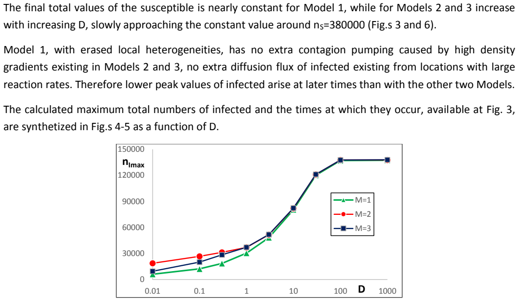
The paper's central claim is that the modified finite volume method it introduces, called Model 2, produces almost the same epidemic evolution as the fully resolved Model 3, except at small diffusion. In Model 2, each coarse control volume is divided into two unlocalized subvolumes representing high- and low-susceptibility patches; only their volume fractions, mutual interface area $A_{12}$, and distance $d_{12}$ are specified. Inter-control-volume diffusion flux is distributed among the subvolumes in proportion to their volume fraction, and intra-control-volume flux is computed from assigned areas and distances, preserving conservation of the transported infected individuals. With hand-picked but non-optimized values $A_{12}=5.1$ and $d_{12}=1.4$, the simulations yield nearly coincident wave speeds, peak infected times and magnitudes, and final susceptible counts for $D \geq 0.3$, and the exact integral relation between total infected and susceptible is satisfied. At small $D$, Model 2 deviates: it produces earlier and higher infected peaks than Model 3, though the final susceptible totals remain close.
Load-bearing premise
The accuracy of Model 2 rests on the assumption that the infected flux entering a coarse cell from its neighbors is shared among that cell's subvolumes purely in proportion to their volume fractions, regardless of where each subvolume sits inside the cell.
Editorial extensions
If this is right
- At moderate and large diffusion (roughly $D \geq 0.3$ in the simulation units), the geometry-free Model 2 can replace the fully resolved Model 3 for predicting total infected, total susceptible, and wave speed.
- The mean-field Model 1 is reliable only when diffusion is large enough to homogenize the infected field; at small and moderate $D$ it underestimates contagion because it averages away high-density patches.
- The exact integral relation between total infected and susceptible (Eq. 8) holds across all models and provides a cheap accuracy check on any numerical solution's integral quantities.
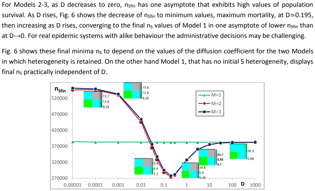
- The final number of susceptibles as a function of $D$ has a minimum near $D \simeq 0.2$ in the heterogeneous models, while the mean-field model predicts a nearly constant final toll; this non-monotonicity is a fingerprint of retained heterogeneity.
Reading between the lines
- If Model 2's parameters were optimized against field data, the fitted $A_{kk'}/d_{kk'}$ values could serve as effective descriptors of unresolved sub-grid contact structure, giving a practical way to infer heterogeneity from outbreak curves.
- The method's assumption that inter-cell flux spreads by volume fraction should fail when subvolumes are strongly segregated within a cell (for example, a high-density patch pressed against a cell face); testing Model 2 against a Model 3 with such a layout would map the limits of the approach.
- The same modified finite volume treatment could be applied to non-epidemic reaction-diffusion systems, such as chemical waves or ecological invasions, wherever small-scale composition is unknown but volume fractions and contact areas can be estimated.
- The reported near-equality of Models 2 and 3 at moderate $D$ may depend on the 1:8 ratio between high- and low-susceptibility volumes; rerunning with different ratios would show whether the method's accuracy scales with heterogeneity contrast.
Signed reviews
Editorial analysis
A structured set of objections, weighed in public.
Referee Report
Summary. The paper defines an SI reaction-diffusion epidemic model with a spatially heterogeneous initial susceptible density and compares three discretizations: Model 1, a coarse-grid mean-field model; Model 2, a modified finite-volume scheme in which each coarse control volume contains two unlocalized subvolumes with assigned sizes, contact areas, and distances; and Model 3, a fully resolved finite-volume model used as reference. The author simulates the spatiotemporal evolution of infected and susceptible densities, reports infection-wave speeds, total infected and susceptible dynamics, and final susceptible counts over a range of diffusion coefficients D. The central claim is that Model 2, despite its loosely defined internal geometry, reproduces Model 3's results very well at moderate diffusion and that all models converge at large D, while Model 1 is accurate only at large D. The paper also presents exact integral relations used to check conservation properties.
Significance. If the central claim is established, the proposed Model 2 would offer a practical way to incorporate short-range heterogeneity in reaction-diffusion systems when detailed geometric information is unavailable, which is relevant to ecological and epidemiological modeling. The paper gives a clearly defined synthetic test problem and provides exact integral relations (Eqs. 8-9) that the numerical schemes satisfy, which is a useful sanity check. The idea of distributing inter-control-volume fluxes among internal subvolumes while preserving conservation is an interesting constructive contribution. However, the current evidence for the central claim is insufficient: the key comparison is visual, the internal geometric parameters are chosen with knowledge of the reference model, and the method's failure at small D is acknowledged but not quantified or bounded.
major comments (5)
- [Section 2.3] The parameters A12=5.1 and d12=1.4 are described as 'non-optimized values, nevertheless guided by similarities with Model 3.' Because these values are chosen using knowledge of the exact geometry of the reference model, the claimed agreement between Models 2 and 3 at moderate D is partly by construction. The paper needs a sensitivity analysis over A12 and d12, or an out-of-sample test on a different heterogeneity configuration, to show that the agreement is an intrinsic property of the method rather than a tuning artifact.
- [Section 4] The text concedes that altering Akk'/dkk' would 'probably break the coincidence existing between Models 2-3' at intermediate D. This admission directly undermines the robustness of the central claim. The authors should quantify the sensitivity of the moderate-D agreement to the geometric parameters and, if the agreement is indeed fragile, temper the claim that Model 2 is a generally reliable substitute when details are unknown.
- [Section 3, Figs. 3-6 and Table I] The 'excellent agreement' between Models 2 and 3 is supported only by qualitative visual comparison of curves. No quantitative error metric (e.g., L1 or L2 differences in nI(t), nS(t), final nS, or wave speed) is provided. Quantitative measures are needed to substantiate the central claim and to allow comparison across D values and across possible parameter choices.
- [Section 4] The paper acknowledges that at small D, Model 2 leads to 'large diffusion too early' and that modifications are needed. Since small D is a substantial part of the parameter range studied, the claim 'excepting at small D, the results of Models 2 and 3 are very similar' leaves the method's validity in exactly the regime where heterogeneity matters most. The authors should either provide a corrected Model 2 variant that also works at small D, or clearly delimit the range of D for which the method is reliable, with quantitative support.
- [Section 2.3, Eq. 6] The key assumption that inter-control-volume flux is distributed among internal subvolumes proportionally to volume fraction, 'irrespective of the location of each δVk inside δV,' is untested. This assumption could be checked by comparing the subvolume-resolved fluxes of Model 3 with those of Model 2 in a post-processing step. Without such a test, the moderate-D agreement may be coincidental rather than a consequence of the modeling ansatz.
minor comments (5)
- [Throughout] The notation is inconsistent: 'M=1', 'M=2', 'M=3' in figures and tables are used interchangeably with 'Model 1', 'Model 2', 'Model 3'. Please standardize the labels throughout.
- [Table II] Table II has no caption or title, making it difficult to interpret. Add a caption describing the entries and their relation to Fig. 7.
- [Section 2.1] The initial condition is described as 'the rectangle approximately centred at (150,1.923)', but the precise cell indices are not given for Models 1 and 3. Specify which control volume is seeded.
- [Section 2.3] The sentence 'The coefficients an of Eq.s 6 and 3 are identical' is unclear because the symbol an is not explicitly defined in Eq. 6. Please define all symbols in Eqs. 5-7.
- [References] Some references are incomplete or inconsistently formatted (e.g., Noble 1974 and Silva 2016 are cited in the text but the full entries are missing from the reference list). Also, the reference to 'Artemov et al. 2009' lists many co-authors; the entry should be checked for completeness.
Circularity Check
No significant circularity: the Model 2 vs Model 3 agreement is a numerical comparison with openly stated geometric inputs, not an algebraic consequence of the inputs.
full rationale
The paper's central claim is an empirical/numerical comparison of three discretizations of the same reaction-diffusion system. Model 2's geometric parameters are not fitted to the reference outputs: the volume fractions δV1=δV/9 and δV2=8δV/9 are 'true' system values, and A12=5.1 and d12=1.4 are explicitly 'non-optimized values, nevertheless guided by similarities with Model 3.' Choosing subvolume sizes and contact parameters from known system geometry is model calibration, not circularity; the matched nI(t), wave speeds, and nSfin(D) curves emerge from solving the balance equations and are not algebraic identities. The flux-redistribution assumption ('irrespective of the location of each δVk inside δV') is stated openly and is an assumption about model error, not a hidden reuse of the target result. The self-citation to Silva 2016 merely supplies the base SI model and is not load-bearing. Finally, the Section 4 admission that changing Akk'/dkk' would 'probably break the coincidence' is a sensitivity/robustness limitation, not evidence that the agreement is equivalent to its inputs by construction. The exact integral relations (Eqs. 8-9) are conservation checks applied equally to all models, and do not force Model 2 to match Model 3.
Assumptions & free parameters
free parameters (4)
- A12 (subvolume contact area in Model 2) =
5.1
- d12 (subvolume distance in Model 2) =
1.4
- kC (contagion coefficient) =
0.015
- mu (mortality coefficient) =
0.25
assumptions (5)
- domain assumption The epidemic contagion rate is bilinear: kC * S * I.
- domain assumption Infected flux is Fickian: proportional to the gradient of I with constant diffusion coefficient D.
- domain assumption The domain is isolated with zero-flux boundaries.
- ad hoc to paper Diffusion flux between control volumes in Model 2 is distributed among internal subvolumes proportionally to subvolume volume fraction, irrespective of location.
- domain assumption The subvolume sizes δV1=δV/9 and δV2=8δV/9 carry the true short-range composition fractions.
invented entities (1)
-
Unlocalized subvolumes δVk inside each control volume
Cite this review
Pith. "Pith review of Model for heterogeneous reaction-diffusion systems with application to one epidemic." pith.science (2026). https://pith.science/paper/XPOWWBZ3
@misc{pith2026190809149,
  author       = {Pith},
  title        = {Pith review of: Model for heterogeneous reaction-diffusion systems with application to one epidemic},
  year         = {2026},
  howpublished = {\url{https://pith.science/paper/XPOWWBZ3}},
  note         = {Machine review of arXiv:1908.09149}
}
read the original abstract
The dynamics of ecological as well as chemical systems may depend on heterogeneous configurations. Heterogeneity in reaction-diffusion systems often increase modelling and simulating difficulties when non-linear effects are present. One synthetic epidemic system with short range heterogeneous composition is modelled and its space-time evolution studied using maximum heterogeneity details. Two other modelling alternatives are applied, one of them using elementary mean-field variables, one other using non-localized geometrical parameters, so avoiding the limitations of the used mean-field model, while keeping significant features of more detailed models. Both the detailed and the mean-field models are solved by means of the standard finite volume method. The model with less defined geometry is solved by means of one modified version of the finite volume method. Simulation results of the three models are compared. At the high diffusion range all models behave similarly. At moderate diffusion fluxes, the numerical results of the model with reduced geometric details are in excellent agreement with the results of the detailed model. The simple mean-field model presents limited accuracy at low and moderate values of the diffusion coefficient.
Figures

Reference graph
Works this paper leans on
-
[1]
Alonso S, Bär M, Kapral R (2009) Effective medium approach for heterogeneous reaction-diffusion media. J. Chem. Phys., 131, 214102. 19 Artemov V, Beale S, Vahl Davis G, Escudier M, Fueyo N, Launder B, Leonardi E, Malin M, Minkowycz W, Patankar S, Pollard A, Rodi W, Runchal A, Vanka S (2009) A tribute to D.B. Spalding and his contributions in science and e...
work page 2009
Reviewed August 14, 2026 · model on record in the stance chip above.
Discussion (0). Continue with ORCID to comment.