REVIEW 3 major objections 4 minor 38 references
Persistent instability in a nonhomogeneous delay differential equation system of the Valsalva maneuver
T0 review · 3 major / 4 minor · reviewed 2026-08-14 · deepseek-v4-flash
Pith's one-line read Blood-pressure-derived forcing widens the stable sink region of a delay-equation Valsalva model while leaving the Hopf threshold unchanged.
desk verdict A correct but standard homogeneous DDE stability analysis attached to a nonhomogeneous numerical map whose central claim is likely contaminated by the artificially extended forcing function. read the letter →
The pith
A machine-rendered reading of the paper's core claim, the machinery that carries it, and where it could break.
The reading
What carries the argument
The carrying object is the characteristic equation $\varphi(\lambda) = \tau_s\lambda + e^{-\lambda D_s} = 0$ for the delayed sympathetic-tone equation, solved through the Lambert W function; its roots determine the homogeneous stability boundaries. The companion mechanism is the forcing pair $f(t)$ and $g(t)$ built from a tenth-degree polynomial fit to one-second moving-average systolic blood-pressure data, which turns the homogeneous system into the nonhomogeneous system $\dot{x} = Ax + Bx_{D_s} + \mathbf{f}$. Numerical solution on a $D_s \times \tau_s$ mesh with a qualitative amplitude-trend classifier then locates the nonhomogeneous boundaries.
What would settle it
Recompute the nonhomogeneous boundary with the forcing functions truncated at the end of the Valsalva maneuver, removing the artificial post-maneuver extension; if the overdamped-sink region no longer extends beyond $\tau_s = eD_s$, or if the POTS subject moves to a different region, the claimed stabilization is an artifact of the constructed input rather than a property of the DDE.
Extended reading notes
Core claim
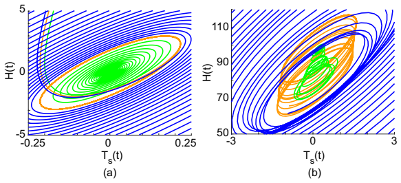
The central claim is that in the nonhomogeneous system the forcing function acts as a stabilizer: the gray overdamped-sink region extends beyond the analytically derived line $\tau_s = eD_s$, the transcritical boundary becomes a curve rather than a line, and the stable-focus region shrinks accordingly, while the Hopf bifurcation line $D_s = \tau_s\pi/2$ and the unstable region occur at the same parameter locations as in the homogeneous system. The authors further claim that the model's classification of the POTS patient in the stable-focus region supports the clinical hypothesis that POTS involves altered, overactive sympathetic nervous system activity.
Load-bearing premise
The stability-boundary shift depends on a 10th-degree polynomial fit to one-second averaged blood-pressure data that was artificially extended after the maneuver; if that extension manufactures oscillations, the widened sink region and the patient classifications are artifacts of the input construction rather than intrinsic dynamics of the delay system.
Editorial extensions
If this is right
- In the two-parameter plane, the stable sink region for the forced system is larger than the homogeneous prediction $\tau_s = eD_s$, meaning some parameter pairs that would oscillate without forcing are stabilized by the blood-pressure input.
- The Hopf bifurcation line $D_s = \tau_s\pi/2$ is unchanged by forcing, so the onset of limit cycles and divergence is governed by the same delay-to-time-scale ratio in both systems.
- A control subject can sit in either the sink or stable-focus region, so stable-focus behavior by itself is not a disease marker; the POTS patient's stable-focus placement is consistent with overactive sympathetic signaling rather than with a limit cycle.
- To stay physiologically relevant, model parameters should be restricted to the sink and stable-focus regions, since limit-cycle and unstable regions are not observed in practice.
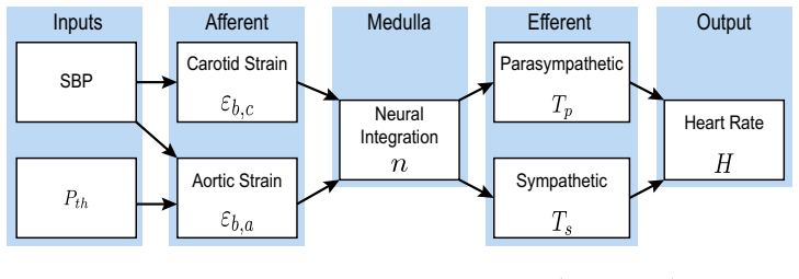
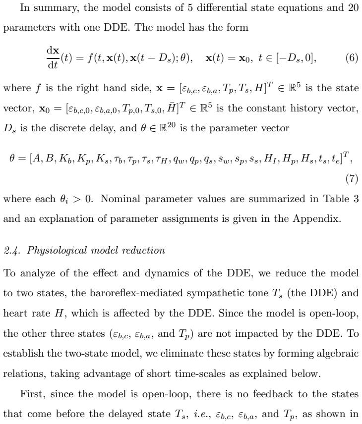
- The reduced two-state model preserves the qualitative stability classification of the full five-state model, so the bifurcation analysis can be carried out on the simpler system.
Reading between the lines
- If the polynomial fit's artificial extension after the maneuver injects a decaying oscillation, the claimed widening of the sink region may be partly an input artifact; a natural test is to rerun the grid with forcing truncated at the end of the maneuver.
- The same stability analysis could be applied to other transient autonomic challenges, such as tilt-table tests, by replacing the Valsalva forcing while keeping the homogeneous characteristic equation fixed.
- Parameter pairs just inside the stable-focus region near the Hopf line predict slowly damped oscillations, so fitting individual patient data there could yield a quantitative metric of sympathetic damping time.
- The boundary shift implies that the effective stabilization depends on the amplitude and shape of the forcing, so constructing forcing from real-time beat-to-beat data rather than a polynomial fit would make the predicted patient classifications testable in clinical recordings.
Signed reviews
Editorial analysis
A structured set of objections, weighed in public.
Referee Report
Summary. This paper studies a two-state reduction of a baroreflex model of the Valsalva maneuver, consisting of a linear delayed differential equation for sympathetic outflow Ts coupled to heart rate H, together with nonhomogeneous forcing terms f(t) and g(t) derived from filtered and polynomial-fitted systolic blood pressure data. For the homogeneous system the authors derive analytical stability boundaries via the Lambert W function, obtaining a real-to-complex root transition at τs = e Ds and an imaginary-axis crossing at Ds = πτs/2. For the nonhomogeneous system they use an algorithmic classification of solution waveforms to claim that the forcing expands the sink region beyond the τs = e Ds line while leaving the limit-cycle and unstable boundaries at the same locations. They then classify two control subjects and one POTS patient as belonging to the sink or stable-focus regions and argue that the model supports the hypothesis of altered sympathetic activity in POTS.
Significance. If the nonhomogeneous stability map were validated, the paper would provide an interesting demonstration that bounded, nonperiodic forcing can shift apparent stability boundaries in a physiological delay differential equation model, and the homogeneous boundary in the (Ds, τs) plane is a clean, correct analytical result. The paper has several strengths: the Lambert-W-based derivation of the homogeneous stability boundaries is careful and reproducible; the reduction from five states to two is clearly documented; and Algorithm 1 is explicit enough to be checked. However, the central claim about the nonhomogeneous system rests on forcing functions constructed with an artificial extension of the data and on an ad-hoc waveform-classification algorithm. Without robustness checks, the claimed stabilization by forcing is not established, and the clinical interpretation for the POTS patient depends on that unvalidated numerical map.
major comments (3)
- [Section 3.1, Eq. (37) and Fig. 9; also Abstract] The transition at τs = e Ds is repeatedly called a 'transcritical bifurcation' (Abstract, Section 3.1, and the caption of Fig. 9). However, for the homogeneous system (21) the origin is the unique equilibrium and remains stable on both sides of this line; what changes is that the two real characteristic roots coalesce and become complex. There is no second equilibrium crossing and no exchange of stability, so this is not a transcritical bifurcation. This mischaracterization propagates to the abstract and conclusions and should be corrected, e.g., by describing it as a node-to-focus transition or a change in the nature of the stable equilibrium.
- [Section 2.4, paragraph after Fig. 5; Section 3.2; Fig. 9b] The central nonhomogeneous result—that the forcing expands the sink region beyond τs = e Ds while preserving the Hopf and unstable boundaries—is produced by Algorithm 1 applied to solutions driven by forcing functions built from a 10th-degree polynomial fit to a one-second moving average of SBP and artificially extended after the maneuver 'to accentuate the oscillatory behavior of the signal if it arises.' Because these forcing functions are bounded, non-decaying, and non-periodic, they can generate oscillatory or decaying-oscillatory transients that Algorithm 1 may attribute to intrinsic DDE stability. As written, the reported boundary shift is indistinguishable from an artifact of the polynomial tail and extension procedure. The authors should repeat the classification with forcing built from the unextended data (or with truncation at several different times), or otherwise demonstrate that the claimed boundary shift is invariant to the extension, or refrain from claiming a stabilizing effect of the forcing.
- [Section 3.2, Algorithm 1] The numerical 'stability regions' for the nonhomogeneous system are defined by counting local extrema of Ts after the maneuver and regressing their amplitudes with ad-hoc thresholds η1 = 0.5, η2 = −10⁻², and μ = 0.8. This classifies transient waveform shapes, not stability in the sense of convergence to an equilibrium; a nonautonomous system with persistent bounded forcing does not possess an equilibrium whose stability can be read from the homogeneous characteristic roots. The paper should justify that the Algorithm-1 boundary corresponds to a dynamically meaningful invariant (e.g., exponential contraction to a bounded attractor) or at least validate the thresholds and the post-maneuver window against problems with known decay rates. Without such validation, the 'stability regions' in Fig. 9b are not tied to the analytical stability theory of Section 3.1.
minor comments (4)
- [Section 3.1, text near Eq. (36)] The sentence 'Substituting λ* into equation (29) and setting λ* ≤ 0 yields' appears to be a typo: the condition is φ(λ*) ≤ 0, not λ* ≤ 0. Please fix the wording.
- [Section 2.4 and Section 3.1] There are two unresolved 'Figure ??' placeholders: one after the description of the SBP polynomial fit and one in the discussion of the Lambert W branches. These should be replaced with the correct figure references.
- [Algorithm 1, step 4] The filtering rule based on |Mi − mi| < 10⁻⁸ is described in prose but the formatting of the vector definitions and loop makes it easy to misread; a numbered or displayed procedure would improve clarity.
- [Table 4] The estimated Ds and τs values for the three subjects are presented without uncertainties or details of how they were estimated; a brief explanation of the estimation procedure would help readers assess the classification claims.
Circularity Check
No significant circularity: the homogeneous stability derivation is self-contained; the nonhomogeneous classification depends on data-derived forcing and hand-set thresholds, but no output is defined in terms of or fitted to the claimed result.
full rationale
The homogeneous analysis in Sec. 3.1 is a genuine derivation: it starts from the DDE (22)-(23), assumes exponential solutions, obtains the characteristic equation phi(lambda) = tau_s lambda + e^{-lambda D_s} = 0 (Eq. 29), solves via the Lambert W function (Eq. 34), and derives the real-root condition e D_s <= tau_s (Eq. 37) and the Hopf line D_s = tau_s pi/2 (Eq. 44). No parameter is fitted to the stability boundary, and no self-citation is load-bearing for those inequalities. The nonhomogeneous results in Sec. 3.2 and Fig. 9b are numerical classifications from Algorithm 1, not analytic predictions, so the serious concerns are whether the classifier thresholds and the artificial extension of the SBP polynomial bias the reported sink/focus/limit-cycle regions. That is a correctness and validity issue, not a circularity: the paper never defines the homogeneous lines in terms of Algorithm 1, and it does not claim the forcing tail was fit to reproduce the stability map. Table 4 reports subject-specific D_s and tau_s without an explicit fitting procedure and defers parameter assignment to Randall et al. [24], but the clinical classification is an interpretation of where those parameter values fall, not an equation-level reduction of the conclusion to its inputs. Under the rule that circularity requires a quotable reduction (Eq. X = Eq. Y by construction, or fitted parameter renamed as prediction), no such reduction is exhibitable here; the artificial-extension and threshold concerns are best scored as modeling risk rather than circularity.
Assumptions & free parameters
free parameters (5)
- Subject-specific sympathetic delay Ds =
S1: 9.2 s, S2: 4.7 s, S3: 5.6 s
- Subject-specific sympathetic time-scale tau_s =
S1: 7.5 s, S2: 5.4 s, S3: 5.2 s
- SBP polynomial coefficients a_0 through a_10 =
Not listed in paper
- Classification thresholds in Algorithm 1 =
eta1=0.5, eta2=-0.01, mu=0.8; also 0.1 s minimum extremum distance and 1e-8 amplitude cutoff
- Moving-average window length for SBP filtering =
1 s
assumptions (6)
- domain assumption Fast baroreceptor and parasympathetic states are in quasi-steady-state (tau_p = 0 and tau_b = 0)
- ad hoc to paper The carotid baroreceptor pathway can be ignored (B = 0)
- domain assumption Sympathetic transmission is a discrete delay Ds
- ad hoc to paper The forcing functions reconstructed from filtered and artificially extended SBP represent physiological input
- standard math The principal branch of the Lambert W function determines stability
- ad hoc to paper The node-focus transition is a transcritical bifurcation and the imaginary-axis crossing is a Hopf bifurcation
Cite this review
Pith. "Pith review of Persistent instability in a nonhomogeneous delay differential equation system of the Valsalva maneuver." pith.science (2026). https://pith.science/paper/GQVUONIN
@misc{pith2026190809371,
  author       = {Pith},
  title        = {Pith review of: Persistent instability in a nonhomogeneous delay differential equation system of the Valsalva maneuver},
  year         = {2026},
  howpublished = {\url{https://pith.science/paper/GQVUONIN}},
  note         = {Machine review of arXiv:1908.09371}
}
read the original abstract
Delay differential equations (DDEs) are widely used in mathematical modeling to describe physical and biological systems. Delays can impact model dynamics, resulting in oscillatory behavior. In physiological systems, this instability may signify (i) an attempt to return to homeostasis or (ii) system dysfunction. In this study, we analyze a nonlinear, nonautonomous, nonhomogeneous open-loop neurological control model describing the autonomic nervous system response to the Valsalva maneuver. Unstable modes have been identified as a result of parameter interactions between the sympathetic delay and time-scale. In a two-parameter bifurcation analysis, we examine both the homogeneous and nonhomogeneous systems. Discrepancies between solutions result from the presence of the forcing functions which stabilize the system. We use analytical methods to determine stability regions for the homogeneous system, identifying transcendental relationships between the parameters. We also use computational methods to determine stability regions for the nonhomogeneous system. The presence of a Hopf bifurcation within the system is discussed and solution types from the sink and stable focus regions are compared to two control patients and a patient with postural orthostatic tachycardia syndrome (POTS). The model and its analysis support the current clinical hypotheses that patients suffering from POTS experience altered nervous system activity.
Figures

Figures from the paper (10 more)





Reference graph
Works this paper leans on
-
[1]
Analysis of a sys tem of linear delay differential equations
Asl, Farshid Maghami and Ulsoy, A Galip. Analysis of a sys tem of linear delay differential equations. J Dyn Syst-T ASME , 125: 215–223,
-
[2]
Modeling bumblebee pop- ulation dynamics with delay differential equations
Banks, H T; Banks, J E; Bommarco, Riccardo; Laubmeier, A N ; Myers, N J; Rundlof, Maj, and Tillman, Kristen. Modeling bumblebee pop- ulation dynamics with delay differential equations. Ecol Model , 351: 14–23, 2017
work page 2017
-
[3]
Differential-Difference Equa- tions
Bellman, Richard and Cooke, Kenneth L. Differential-Difference Equa- tions. Elsevier Science, United Kingdom, 1963
work page 1963
-
[4]
Bi, Ping and Ruan, Shigui. Bifurcations in delay different ial equa- tions and applications to tumor and immune system interacti on models. SIAM J Appl Dyn Sys , 12: 1847–1888, 2013. 34
work page 2013
-
[5]
Medical Physiology: A Cellular and Molecular Approach
Boron, Walter F and Boulpaep, Emil L. Medical Physiology: A Cellular and Molecular Approach . Elsevier Inc., third edition, 2017
work page 2017
-
[6]
Two-param eter bifur- cation analysis of limit cycles of a simplified railway wheel set model
Cheng, Lifang; Xiukun, Wei, and Cao, Hongjun. Two-param eter bifur- cation analysis of limit cycles of a simplified railway wheel set model. Nonlinear Dyn , 93: 2415–2431, 2018
work page 2018
-
[7]
Delay-induced oscillatory dynamics of tumour-immune syst em interac- tion
d’Onofrio, Alberto; Gatti, Francesca; Cerrai, Paola, a nd Freschi, Luca. Delay-induced oscillatory dynamics of tumour-immune syst em interac- tion. Math Comput Model , 51: 572–591, 2010
work page 2010
-
[8]
Numerica l bifurcation analysis of delay differential equations using DDE-BIFTOOL
Engelborghs, K; Luzyanina, T, and Roose, Dirk. Numerica l bifurcation analysis of delay differential equations using DDE-BIFTOOL. ACM Trans Math Solftw , 28: 1–21, 2002. DOI: 10.1145/513001.513002
Show all 38 references
-
[9]
Implementing Radau IIA metho ds for stiff delay differential equations
Guglielmi, N and Hairer, E. Implementing Radau IIA metho ds for stiff delay differential equations. Computing, 67 (1), 2001. DOI: 10.1007/s006070170013
2001 doi
-
[10]
Guyton and Hall Textbook of Medical Physiology
Hall, John E. Guyton and Hall Textbook of Medical Physiology . Elsevier, Inc., Philadelphia, PA, thirteenth edition, 2016
2016
-
[11]
Arteria l, cere- brospinal, and venous pressures in man during cough and stra in
Hamilton, W F; WoodBury, R A, and Jr.Harper, H T. Arteria l, cere- brospinal, and venous pressures in man during cough and stra in. Am Heart J , 27 (6): 871, 1943. DOI: 10.1016/S0002-8703(44)90319-4
1943 doi
-
[12]
Cli- mate models with delay differential equations
Keane, Andrew; Krauskopt, Bernd, and Postlethwaite, C laire M. Cli- mate models with delay differential equations. Chaos, 27: 114309, 2017. DOI: 10.1063/1.5006923. 35
2017 doi
-
[13]
Bifurcation analysi s of delay- induced resonances of the El Ni˜ no Southern Oscillation
Krauskopf, Bernd and Sieber, Jan. Bifurcation analysi s of delay- induced resonances of the El Ni˜ no Southern Oscillation. Proc Math Phys Eng Sci , 420 (2169): 1–18, 2014
2014
-
[14]
Delay Differential Equations with Applications in Popu- lation Dynamics , volume 191
Kuang, Yang. Delay Differential Equations with Applications in Popu- lation Dynamics , volume 191. Academic Press, San Diego, CA, 1993
1993
-
[15]
A human cardiopulmonary system model applied to the analysis of the Valsalva maneuver
Lu, K; Clark Jr., J W; Ghorbel, F H; Ware, D L, and Bidani, A . A human cardiopulmonary system model applied to the analysis of the Valsalva maneuver. Am J Physiol Heart Circ Physiol , 281 (6): H2661– H2679, 2001. DOI: 10.1093/cvr/23.8.683
2001 doi
-
[16]
Numerical bifurcation analysis of immunological models with time del ays
Luzyanina, Tatyana; Roose, Dirk, and Bocharov, Gennad y. Numerical bifurcation analysis of immunological models with time del ays. J Comp Appl Math , 184: 165–176, 2005
2005
-
[17]
Modeling the afferent dynamics of the baroreflex control syste m
Mahdi, Adam; Sturdy, Jacob; Ottesen, Johnny T, and Oluf sen, Mette S. Modeling the afferent dynamics of the baroreflex control syste m. PLoS Comput Biol , 9 (12): 1–18, 2013. DOI: 10.1371/journal.pcbi.1003384
2013 doi
-
[18]
Mathema tical mod- els and software tools for the glucose-insulin regulatory s ystem and diabetes: an overview
Makroglou, Athena; Li, Jiaxu, and Kuang, Yang. Mathema tical mod- els and software tools for the glucose-insulin regulatory s ystem and diabetes: an overview. Apl Num Math , 56: 559–573, 2006
2006
-
[19]
Mathematical ana lysis of delay differential equation models of HIV-1 infection
Nelson, Patrick and Perelson, Alan S. Mathematical ana lysis of delay differential equation models of HIV-1 infection. Math Biosci , 179: 73– 94, 2002
2002
-
[20]
Modeling Heart Rate Regulation by the Baroreflex
Olsen, Christian Haargaard. Modeling Heart Rate Regulation by the Baroreflex. Thesis, North Carolina State University, 2014. 36
2014
-
[21]
Blood pressure and blood fl ow variation during postural change from sitting to standing: model devel- opment and validation
Olufsen, Mette S; Ottesen, Johnny T; Tran, Hien T; Ellwe in, Laura M; Lipsitz, Lewis A, and Novak, Vera. Blood pressure and blood fl ow variation during postural change from sitting to standing: model devel- opment and validation. J Appl Physiol , 99 (4): 1523–1537, 2005. DOI: ...
2005
-
[22]
Modelling of the baroreflex-feedbac k mecha- nism with time-delay
Ottesen, Johnny T. Modelling of the baroreflex-feedbac k mecha- nism with time-delay. J Math Biol , 36 (1): 41–63, 1997. DOI: 10.1007/s002850050089
1997 doi
-
[23]
The utility of Valsalva maneuver in the diagnoses of orthostatic disord ers
Palamarchuk, Iryna S; Baker, Jacquie, and Kimpinski, K urt. The utility of Valsalva maneuver in the diagnoses of orthostatic disord ers. Am J Physiol Regul Integr Comp Physiol , 310 (3): R243–252, 2016. DOI: 10.1152/ajpregu.00290.2015
2016
-
[24]
A model-based analysis of auto nomic nervous function in response to the Valsalva maneuver
Randall, Eric Benjamin; Billeschou, Anna; Brinth, Lou ise S; Mehlsen, Jesper, and Olufsen, Mette S. A model-based analysis of auto nomic nervous function in response to the Valsalva maneuver. J Appl Physiol ,
-
[25]
Dyna mics of a diffusion reaction prey-predator model with delay in prey: effe cts of delay and spatial components
Rao, Feng; Casillo-Chavez, Carlos, and Kang, Yun. Dyna mics of a diffusion reaction prey-predator model with delay in prey: effe cts of delay and spatial components. J Math Anal Appl , 461: 1177–1214, 2018
2018
-
[26]
Continuation and bifurcation analysis of delay differential equations , pages 359–394
Roose, Dirk and Szalai, Robert. Continuation and bifurcation analysis of delay differential equations , pages 359–394. Springer, Dordrecht, 2007
2007
-
[27]
On the zeros of transcende ntal functions 37 with applications to stability of delay differential equatio ns with two delays
Ruan, Shigui and Wei, Junjie. On the zeros of transcende ntal functions 37 with applications to stability of delay differential equatio ns with two delays. Dyn Cont Disc Imp Syst , 10: 863–874, 2003
2003
-
[28]
Robust stabili ty analysis of linear time-delay systems by Lambert W function: some extreme point results
Shinozaki, Hiroshi and Mori, Takehiro. Robust stabili ty analysis of linear time-delay systems by Lambert W function: some extreme point results. Automatica, 42: 1791–1799, 2006
2006
-
[29]
Stability and stabilization of systems w ith time delay
Sipahi, Rifat; Niculescu, Silviu-iulian; Abdallah, C haouki T; Micheils, Wim, and Gu, Keqin. Stability and stabilization of systems w ith time delay. IEEE Contr Syst Mag , 31: 38–65, 2011
2011
-
[30]
Conti nuation of bifurcations in periodic delay-differential equations usin g characteristic matrices
Szalai, Robert; Stepan, Gabor, and Hogan, S John. Conti nuation of bifurcations in periodic delay-differential equations usin g characteristic matrices. SIAM J Sci Comput , 28 (4): 1301–1317, 2006
2006
-
[31]
Age- predicted maximal heart rate revisited
Tanaka, Hirofumi; Monohan, Kevin D, and Seals, Douglas R. Age- predicted maximal heart rate revisited. J Am Coll Cardiol , 37 (1): 153–156, 2001
2001
-
[32]
Delay equation ana lysis of human respiratory stability
Vielle, Bruno and Chauvet, Gilbert. Delay equation ana lysis of human respiratory stability. Math Biosci , 152: 105–122, 1998
1998
-
[33]
Autonomic testing: common techniques and clinical applications
Weimer, Louis H. Autonomic testing: common techniques and clinical applications. The Neurologist, 16 (4): 215–222, 2010
2010
-
[34]
Circulatory model of bar o- and cardio- pulmonary reflexes
Wesseling, K H and Settels, J J. Circulatory model of bar o- and cardio- pulmonary reflexes. In Blood Pressure and Heart Rate Variability , vol- ume 4, pages 56–67. IOS Press, Amsterdam, The Netherlands, 1 993
-
[35]
The smallest chemical reaction syste m with bista- bility
Wilhelm, Thomas. The smallest chemical reaction syste m with bista- bility. BMC Syst Biol , 9, 2009. DOI: 10.1186/1752-0509-3-90. 38
2009 doi
-
[36]
Solution of a system of linear delay differen- tial equations using the matrix Lambert function
Yi, Sun and Ulsoy, A Galip. Solution of a system of linear delay differen- tial equations using the matrix Lambert function. In Proc Am Control Conf, pages 2433–2438. IEEE, 2006. DOI: 10.1109/ACC.2006.1656 585. 39
2006
-
[2003]
DOI: 10.1115/1.1568121
-
[2019]
DOI: 10.1152/japplphysiol.00015.2019
2019
Reviewed August 14, 2026 · model on record in the stance chip above.
Discussion (0). Continue with ORCID to comment.