A linear system for pipe flow stability analysis allowing for boundary condition modifications

Martin Skote; M. Malik

REVIEW 3 major objections 4 minor 39 references

A linear system for pipe flow stability analysis allowing for boundary condition modifications

T0 review · 3 major / 4 minor · reviewed 2026-08-14 · deepseek-v4-flash

Challenge this review Re-run · record.json Download PDF Read on arXiv ↗ Review JSON

Pith's one-line read This paper derives a two-variable spectral system for pipe-flow stability that fixes the centreline regularity conditions once, so wall boundary conditions can be swapped without reformulating the operators, while matching reference…

desk verdict A genuinely accurate and new spectral formulation for pipe flow, but the code's undocumented eigenvalue filter overstates the 'spectrum' claim. read the letter →

arxiv 1908.09626 v1 pith:MJNBV2D5 submitted 2019-08-18 math.NA cs.CEcs.NAphysics.flu-dyn

M. Malik , Martin Skote This is my paper · ORCID

classification math.NAcs.CEcs.NAphysics.flu-dyn MSC 65M7076E0565L15

keywords pipeflowstabilitylinearspectralcollocationcentrelineregularityanalyticansatzalgebraicgrowthoptimaldisturbancescircular

verification ladder T0 review T1 audit T2 compute T3 formal

The pith

A machine-rendered reading of the paper's core claim, the machinery that carries it, and where it could break.

The reading

The paper sets out a spectral method for the linear stability of flow through a circular pipe that keeps the accuracy of the best existing approach while making one previously rigid part of the calculation flexible: the wall boundary condition. The state is written in two unknowns, a factored radial velocity and a factored radial vorticity, chosen so that both are analytic in the squared radius y=r². The regular singularity at the pipe centre then yields exactly the right number of regularity conditions to complement the wall conditions and make the eigenvalue problem well posed, and those conditions are derived once and for all. For axisymmetric, axially constant disturbances the computed eigenvalues agree with the analytical characteristic relations to about 14 digits. If the claim holds, the same equations can be reused with slip, permeable, compliant, or time-dependent walls without re-deriving the stability operators.

What carries the argument

The load-bearing object is the pair (φ, Ω) of factored radial velocity and radial vorticity, together with the coordinate change y=r². Under the standard power-law centreline ansatz, φ and Ω are analytic in y near the centre, so ordinary Chebyshev polynomials of all orders can represent them. The pipe centre is a regular singularity — a point where the coefficient of the highest derivative vanishes, allowing the equations to admit non-analytic branches — and its pole multiplicity is such that the regularity limits of the equations, plus one differentiated equation, produce exactly three centreline conditions for each sixth-order case. That exact count is what lets the three wall conditions be imposed directly on the unknowns, so different wall laws can be substituted without changing the operators.

What would settle it

Solve the same linear stability problem with an independent discretisation that does not impose the analyticity-in-y ansatz — for example, a high-order finite-difference scheme in the original radial coordinate r on a very fine grid, allowing non-analytic centreline behaviour — and compare the full spectra. If any eigenvalue appears there that the present regularity conditions exclude, especially at high azimuthal wavenumber |n| or high axial wavenumber α, the ansatz has discarded a physical mode and the central claim fails; if none appears, the regularity conditions are confirmed to cut exactly the spurious branches.

Watch

Extended reading notes

Core claim

The central claim is that the linearised disturbance equations for pipe flow can be reduced to a sixth-order system in two unknowns — or a fourth-order system for the axisymmetric, axially constant case — with the wall boundary conditions imposed directly on the unknowns rather than built into the basis functions. The unknowns are chosen so that, after factoring out the known power-law behaviour at the centreline, they are analytic functions of y=r². The regular singularity at y=0 has a pole multiplicity that supplies exactly the missing number of centreline conditions: requiring all y-multiplied operator terms to vanish there gives two regularity conditions, and one further condition obtained by differentiating the governing equation ensures fourth-order differentiability of the leading unknown. The resulting spectra match the established high-accuracy benchmark, and in the special case of axisymmetric axially constant modes the eigenvalues match the roots of the analytical characteristic equations to about 14 digits. In the inviscid limit for axially constant modes, the same working variables give an explicit solution with linear-in-time growth of streamwise velocity, reproducing the counter-rotating vortex and streak patterns familiar from plane shear flows.

Load-bearing premise

The derivation assumes every physical disturbance is analytic in r² at the pipe centre once the known power-law factor is removed; if a genuine mode has fractional-power or logarithmic centreline behaviour, the regularity conditions imposed here would delete it from the spectrum.

Editorial extensions

If this is right

The same system of equations can be applied to a range of wall conditions (slip, permeable, compliant, time-dependent) by changing only the boundary rows, not the formulation.
Reference-level accuracy is reached with modest discretization — a 93-by-93 system at N=48 in the standard test cases — and the y-stretching map controls round-off for large axial wavenumber and Reynolds number.
In the axisymmetric, axially constant case, the computed eigenvalues match the analytical characteristic relations to about 14 digits, providing a clean validation benchmark.
The inviscid axially constant analysis gives an explicit solution φ(t,y)=φ0(y), Ω(t,y)=Ω0(y)−2in U_y t φ0(y), showing algebraic growth and optimal vortex/streak patterns like those in plane shear flows.
The pole-counting argument guarantees the conditions are neither under- nor over-specified, so the method does not introduce spurious spectral branches through incorrect regularity treatment.

Reading between the lines

Editorial extensions of the paper, not claims the author makes directly.

If the centreline analyticity assumption transfers, the same regularity-counting strategy should work for other radially inhomogeneous base flows (annular pipes, swirling pipe flow, heated or stratified pipes), because the pole-counting argument is tied to the structure of the singularity, not to the no-slip law.
The boundary-condition flexibility invites a concrete test: implement the same operators with a slip-length or suction/blowing condition and compare against an independent solver; agreement would confirm that the claimed flexibility is real, and disagreement would localise the failure in the regularity conditions.
The explicit inviscid solution implies a quantitative prediction for optimal streaks — their wall distance should shrink as the azimuthal wavenumber n grows, since v'=r^l φ0 peaks nearer the wall — which could be checked against nonlinear DNS at moderate Reynolds numbers.
A practical consequence the authors do not spell out: users must apply the stretching map for large α or Re because φ and Ω may develop boundary-layer behaviour at the centre; the transition point could be detected by monitoring the condition number of the discretised operator.

Share X Bluesky LinkedIn Reddit HN

Signed reviews

No signed human review yet.

Editorial analysis

A structured set of objections, weighed in public.

Desk editor's note, referee report, and a circularity audit.

Desk Editor's Note

read the letter

The two things to know: the paper actually delivers a new spectral formulation for pipe flow stability that matches Meseguer-Trefethen accuracy with a simpler, BC-flexible structure, and it prints the full MATLAB code. The catch is that the code contains a filter that silently drops eigenvalues, so the 'spectrum' shown is a subset, and the text never tells you.

What's genuinely good: the 2-tuple analytic-in-y formulation is new, and the regularity argument based on pole multiplicity is a real contribution. The validation is strong — Table 1 agrees with three independent codes at 8–14 digits, and Table 2 nails the alpha=n=0 characteristic roots to ~14 digits. The inviscid optimal-growth section is a clean, parameter-free derivation that reproduces the lift-up/streak picture without viscosity. That is solid work.

The soft spots are real but not fatal. The filter is the big one: in Appendix B, after solving the generalized eigenproblem, only eigenvalues with -imag(omega) <= alpha (or <=1 for alpha<1) are kept. The body text does not mention this anywhere. As a result, the claim 'the system produces a spectrum' is overstated, and Figures 1 and 2 show only the filtered subset. The validation tables are not affected, but the reader of the paper has no way to know whether the discarded region is physical or spurious. That is a gap that needs to be fixed, either by documenting and justifying the threshold or by showing the discarded modes are spurious.

The boundary-condition flexibility is asserted but never demonstrated: no example with a non-no-slip wall condition appears, so the main advertised advantage remains unproven. Also, the condition-number sentence in Section 3.2 contradicts its own numbers: cond ~10^18 for the present system vs ~10^21 for Burridge-Drazin means the present system is less, not 'much closer', to singularity. Minor wording issue, but confusing.

Who is this for: anyone working on linear or nonmodal stability of pipe flow, and anyone building spectral methods with arbitrary boundary conditions. It deserves a serious referee — the core method is sound and the code is transparent enough that the issues are discoverable. I'd suggest asking the authors to document the mode-selection filter, demonstrate the BC flexibility with one worked example, and fix the condition-number sentence.

Referee Report

3 major / 4 minor

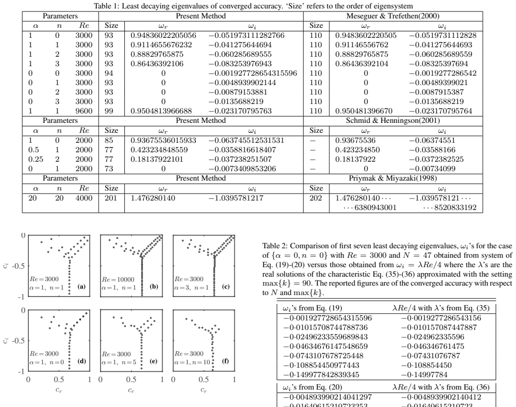
Summary. This manuscript proposes a spectral collocation formulation for the linear stability of Hagen-Poiseuille pipe flow. The authors use the Priymak-Miyazaki ansatz to factor out the centerline power-law behavior of the perturbation velocities, introduce analytic variables φ and Ω in the radial variable y=r², and derive the governing equations (15)-(20) together with the centerline regularity conditions (22)-(27). The claimed advantages are spectral accuracy comparable to Meseguer & Trefethen and the ability to impose different wall boundary conditions directly on the unknowns without reformulating the operators. Validation is provided through agreement with eigenvalues from Meseguer & Trefethen, Schmid & Henningson, and Priymak & Miyazaki in Table 1, and with the exact characteristic roots of the α=n=0 Stokes modes in Table 2. The paper also derives an inviscid algebraic-growth problem in §4 and shows the associated optimal vortex and streak patterns.

Significance. The core technical contribution is plausible, and the numerical validation is strong where it applies. Table 1 shows agreement to 8-14 significant digits against three independent codes, and Table 2 is a clean internal consistency check against exact characteristic relations to about 14 digits. The inviscid optimal-growth derivation in §4 is parameter-free and reproduces the known lift-up/streak phenomenology without fitted constants. The inclusion of the complete MATLAB code in Appendix B is also a practical strength. However, the central claim that the system produces a spectrum as accurate as Meseguer & Trefethen is not supported for the full spectrum, because the code silently discards all eigenvalues whose decay rate exceeds α (or 1). The significance of the paper therefore depends on either demonstrating that the discarded modes are spurious or, if they are physical, restricting all claims to the least-decaying part of the spectrum.

major comments (3)

[Appendix B] Appendix B contains an undocumented filter that removes eigenvalues before the reported spectra are produced. In both the n≠0 block and the n==0 block, after solving the generalized eigenproblem, the code executes `ok=((imag(e)>-1*al)&(al>=1))|((imag(e)>-1)&(al<1)); e=e(ok); q=q(:,ok)`. This discards every mode with decay rate -Im(ω) > α for α≥1, and -Im(ω) > 1 for α<1; no part of §3.1 or §3.2 describes this operation. The filter is not merely removing numerical noise: for the α=n=0 case, the exact characteristic relations (35)-(36) have infinitely many physical roots with -Im(ω) growing without bound, so the code demonstrably deletes physical Stokes modes. Consequently, the abstract's unqualified claim that the system produces a spectrum as accurate as Meseguer & Trefethen is not supported; the precise statement is that it computes a decay-rate-limited subset. The authors should either remove the filter and compare the complete spectra with reference codes, show that the discarded modes are spurious, or explicitly and consistently restate the claim for the least-decaying part of the spectrum.
[§3.2] The statement that all 41 eigenvalues listed in [21] matched at similar accuracy is not documented. Table 1 lists only the least-decaying eigenvalue for each parameter set, so the reader cannot see which 41 modes were compared, what threshold was used, or whether any of them lay in the region removed by the Appendix B filter. Because this comparison is the main evidence for the headline accuracy claim, the authors should tabulate or plot the complete comparison, including the decay rates of the compared modes.
[§1 and §5] The advertised advantage over Meseguer & Trefethen, namely that boundary conditions can be modified without changing the formulation, is asserted but never demonstrated. All computed results use the no-slip conditions (21); no example with a different wall condition, such as slip, transpiration, or a time-dependent condition, is given. Since this flexibility is a central contribution of the paper, at least one demonstration with a non-no-slip boundary condition, ideally with a comparison against an independent method for that condition, is needed before the claim can be evaluated.

minor comments (4)

[§4, Eq. (49)] In the display following Eq. (48), the upper limit of the integration appears as y, although y is the integration variable; this should presumably be 1.
[§3.2] The paragraph comparing condition numbers refers to Eqs. (42)-(42); the second equation number should be (43).
[§2.2] There is a typo in the sentence 'such requirement is satisfied by the the analytic Jν'; the duplicated 'the' should be removed.
[Appendix B] The option `opts.tol=1e-21` asks for a tolerance far below double-precision machine epsilon; this cannot improve the computed eigenvalues and should either be removed or explained in a comment.

Circularity Check

0 steps flagged · score 1.0 of 10

No significant circularity: the derivation is self-contained from the stated Priymak–Miyazaki analyticity ansatz, with validations against independent external benchmarks and an internal exact-roots consistency check.

full rationale

The paper's central derivation takes the Navier–Stokes equations and an explicitly stated analyticity ansatz (Eqs. 7–8) and manipulates them into the linear systems (15)–(20). The regularity conditions (22)–(27) are derived within the paper from the requirement that analytic functions have O(1) derivatives at y=0; they are not imported from an author-specific uniqueness theorem. The accuracy claims are benchmarked against eigenvalue tables from Meseguer & Trefethen, Schmid & Henningson, and Priymak & Miyazaki, which are independent external groups and not fitted inputs. Table 2 compares spectral-collocation eigenvalues with power-series roots of the same characteristic equations; this is an internal consistency check of the numerical solver against an exact solution of the same ODE system, not a circular prediction. Section 4's optimal-growth derivation is parameter-free, following Ellingsen–Palm algebra from the inviscid limit without fitted constants. The self-citations present (Refs. 20, 23, 36) are not load-bearing: Ref. 20 is a supporting remark on velocity behavior, Ref. 23 is an example of time-dependent boundary conditions, and Ref. 36 is a 'see also' for an established variational method. One non-circular concern: the Appendix B code contains an undocumented eigenvalue filter (`ok=((imag(e)>-1*al)&(al>=1))|((imag(e)>-1)&(al<1))`) that discards high-decay modes, and the body of the paper never mentions this selection. This could affect the completeness of the displayed spectra, but it is a reproducibility/completeness issue rather than circularity, since the retained results are not forced by construction from the filter.

Assumptions & free parameters 4 free parameters · 6 assumptions · 0 invented entities

The method leans on the Priymak-Miyazaki centerline analyticity ansatz (Eqs. 7-8) as its main external input; the regularity-condition construction and the code's mode-selection threshold are ad hoc to this paper, and the remaining axioms are standard math and the standard Hagen-Poiseuille setup. No physical constant is fitted to data: the eigenvalue comparisons and the optimal-growth patterns are parameter-free outputs. The only hand-tuned quantities are numerical resolution parameters (grid stretching, mode filter, series truncation, collocation order).

free parameters (4)

Grid-stretching parameter a = a=2 for n≤5; a=3 for n>5.
Hand-tuned in Section 3.1 ('a=2 gives best result, whereas a=3 works well for n>5'). Discretization parameter for Eq. (41b); it clusters collocation points near y=0 and does not enter the physics. Reported eigenvalues are converged with respect to it.
Mode-filter threshold in the code = imag(ω) > -α if α≥1, else imag(ω) > -1.
Ad hoc post-processing cutoff in Appendix B that restricts the modes retained for display and refinement; undocumented in the main text.
Characteristic-series truncation max{k} = 90.
Series cutoff in Eqs. (35)-(36) used for the Table 2 validation; the paper checked max{k}=89 versus 90 and N=46 versus 47 and reports only digits stable across both.
Collocation order N = 47 to 201 depending on the case.
Resolution parameter selected per case (Section 3.1 and code header). Convergence is demonstrated by matching reference values in Table 1; not a fitted physics parameter.

assumptions (6)

domain assumption Priymak-Miyazaki centerline ansatz (Eqs. 7-8): perturbation velocities scale as r^(|n|-1) times functions analytic in r²; all physical eigenmodes satisfy this.
Load-bearing centerline modeling assumption taken from Ref. [19]. The regularity conditions in Section 2.2 are derived from it. If a physical mode had non-analytic centerline behavior, the spectrum would be incomplete. It is validated indirectly by agreement with Meseguer-Trefethen and with the exact roots in Table 2, not proven.
domain assumption Hagen-Poiseuille base flow U=1-r², incompressible Newtonian fluid, and the Fourier ansatz exp[i(αx+nθ-ωt)] for perturbations.
Standard setup of the problem stated in Section 2, Eq. (1); all derived systems (Eqs. 15-20) are specific to this mean flow.
ad hoc to paper Regularity conditions obtained by requiring y-multiplied operator terms to vanish at y=0 (Eqs. 22-27), with the third condition from the once-differentiated governing equation; pole multiplicity yields exactly the needed number of conditions.
Novel counting argument in Section 2.2. It presupposes analyticity of φ and Ω in y and that the limit conditions eliminate exactly the spurious non-analytic branches. Verified numerically through the validation tables, but not proven rigorously.
ad hoc to paper The code-level mode filter keeps only modes with imag(ω) > -α for α≥1 and imag(ω) > -1 for α<1; discarded modes are assumed spurious or irrelevant.
Appendix B 'ok=...' line. The threshold is not stated or justified in the main text and determines which eigenvalues appear in Fig. 1; it does not affect the Table 1 comparisons of least-decaying modes.
standard math Sturm-Liouville theory applies to the α=n=0 Stokes operators: real eigenvalues, orthogonal eigenfunctions, monotone decay (Section 2.3).
Standard result for self-adjoint Stokes operators referenced to Refs. [27,29]; used to claim no transient growth for α=n=0 superpositions.
standard math Spectral collocation in the mapped coordinate y (Eq. 41) converges, and the QZ and EIGS solvers produce the stated digits in double precision.
Numerical method of Section 3.1; convergence is evidenced by N-independence of the reported digits and by agreement with three independent codes.

how reviews work

0 comments

Cite this review

Pith. "Pith review of A linear system for pipe flow stability analysis allowing for boundary condition modifications." pith.science (2026). https://pith.science/paper/MJNBV2D5

@misc{pith2026190809626,
  author       = {Pith},
  title        = {Pith review of: A linear system for pipe flow stability analysis allowing for boundary condition modifications},
  year         = {2026},
  howpublished = {\url{https://pith.science/paper/MJNBV2D5}},
  note         = {Machine review of arXiv:1908.09626}
}

read the original abstract

An accurate system to study the stability of pipe flow that ensures regularity is presented. The system produces a spectrum that is as accurate as Meseguer \& Trefethen (2000), while providing flexibility to amend the boundary conditions without a need to modify the formulation. The accuracy is achieved by formulating the state variables to behave as analytic functions. We show that the resulting system retains the regular singularity at the pipe centre with a multiplicity of poles such that the wall boundary conditions are complemented with precisely the needed number of regularity conditions for obtaining unique solutions. In the case of axisymmetric and axially constant perturbations the computed eigenvalues match, to double precision accuracy, the values predicted by the analytical characteristic relations. The derived system is used to obtain the optimal inviscid disturbance pattern, which is found to hold similar structure as in plane shear flows.

Figures

Figures reproduced from arXiv: 1908.09626 by the authors.

**Figure 2.** Comparison of spectra and eigenfunctions from the present formula [PITH_FULL_IMAGE:figures/full_fig_p008_2.png] view at source ↗

**Figure 3.** The inviscid initial (left) and the instantaneous velocity patterns at a [PITH_FULL_IMAGE:figures/full_fig_p009_3.png] view at source ↗

Discussion (0). Continue with ORCID to comment.

Reference graph

Works this paper leans on

39 extracted references · 39 canonical work pages

[21]

Meseguer, L

A. Meseguer, L. Trefethen, A spectral petrov-galerkin formulation for pipe ﬂow I: linear stability and transient growth, Tech. rep., Oxford Uni- versity Computing Laboratory (2000)

work page 2000
[1]

Itano, S

T. Itano, S. Toh, The dynamics of bursting process in wall turbulence, Journal of the Physical Society of Japan 70 (3) (2001) 703–716 (2001)

work page 2001
[2]

T. M. Schneider, B. Eckhardt, J. A. Yorke, Turbulence transition and the edge of chaos in pipe ﬂow, Physical review letters 99 (3) (2007) 034502 (2007)

work page 2007
[3]

N. B. Budanur, B. Hof, Complexity of the laminar-turbulent boundary in pipe ﬂow, Physical Review Fluids 3 (5) (2018) 054401 (2018)

work page 2018
[4]

Böberg, U

L. Böberg, U. Brosa, Onset of turbulence in a pipe, Zeitschrift für Natur- forschung A 43 (8-9) (1988) 697–726 (1988)

work page 1988
[5]

K. M. Butler, B. F. Farrell, Three-dimensional optimal perturbations in viscous shear ﬂow, Physics of Fluids A: Fluid Dynamics 4 (8) (1992) 1637–1650 (1992)

work page 1992
[6]

L. N. Trefethen, A. E. Trefethen, S. C. Reddy, T. A. Driscoll, Hydrody- namic stability without eigenvalues, Science 261 (5121) (1993) 578–584 (1993)

work page 1993
[7]

P. J. Schmid, D. S. Henningson, Optimal energy density growth in hagen– poiseuille ﬂow, Journal of Fluid Mechanics 277 (1994) 197–225 (1994)

work page 1994

Show all 39 references

[8]

P. J. Schmid, Nonmodal stability theory, Annu. Rev. Fluid Mech. 39 (2007) 129–162 (2007)

2007
[9]

Gavarini, A

M. Gavarini, A. Bottaro, F. Nieuwstadt, The initial stage of transition in pipe ﬂow: role of optimal base-ﬂow distortions, Journal of Fluid Mechan- ics 517 (2004) 131–165 (2004)

2004
[10]

K. C. Sahu, R. Govindarajan, Stability of ﬂow through a slowly diverging pipe, Journal of Fluid Mechanics 531 (2005) 325–334 (2005)

2005
[11]

S. Loh, H. Blackburn, Stability of steady ﬂow through an axially corru- gated pipe, Physics of Fluids 23 (11) (2011) 111703 (2011)

2011
[12]

Pruša, On the inﬂuence of boundary condition on stability of hagen– poiseuille ﬂow, Computers & Mathematics with Applications 57 (5) (2009) 763–771 (2009)

V . Pruša, On the inﬂuence of boundary condition on stability of hagen– poiseuille ﬂow, Computers & Mathematics with Applications 57 (5) (2009) 763–771 (2009)

2009
[13]

Lessen, S

M. Lessen, S. G. Sadler, T.-Y . Liu, Stability of pipe poiseuille ﬂow, The Physics of Fluids 11 (7) (1968) 1404–1409 (1968)

1968
[14]

Burridge, P

D. Burridge, P. Drazin, Comments on â ˘AIJstability of pipe poiseuille ﬂowâ ˘A˙I, The Physics of Fluids 12 (1) (1969) 264–265 (1969)

1969
[15]

Salwen, C

H. Salwen, C. E. Grosch, The stability of poiseuille ﬂow in a pipe of circular cross-section, Journal of Fluid Mechanics 54 (1) (1972) 93–112 (1972)

1972
[16]

Salwen, F

H. Salwen, F. W. Cotton, C. E. Grosch, Linear stability of poiseuille ﬂow in a circular pipe, Journal of Fluid Mechanics 98 (2) (1980) 273–284 (1980)

1980
[17]

Oâ ˘A ´Zsullivan, K

P. Oâ ˘A ´Zsullivan, K. Breuer, Transient growth in circular pipe ﬂow. I. lin- ear disturbances, Physics of ﬂuids 6 (11) (1994) 3643–3651 (1994)

1994
[18]

Thomas, A

C. Thomas, A. Bassom, P. Blennerhassett, The linear stability of oscillat- ing pipe ﬂow, Physics of Fluids 24 (1) (2012) 014106 (2012)

2012
[19]

Priymak, T

V . Priymak, T. Miyazaki, Accurate navier–stokes investigation of tran- sitional and turbulent ﬂows in a circular pipe, Journal of Computational Physics 142 (2) (1998) 370–411 (1998)

1998
[20]

M. R. Khorrami, M. R. Malik, R. L. Ash, Application of spectral colloca- tion techniques to the stability of swirling ﬂows, Journal of Computational Physics 81 (1) (1989) 206–229 (1989)

1989
[22]

Meseguer, L

A. Meseguer, L. N. Trefethen, Linearized pipe ﬂow to reynolds number 107, Journal of Computational Physics 186 (1) (2003) 178–197 (2003)

2003
[23]

Malik, M

M. Malik, M. Skote, R. Bouffanais, Growth mechanisms of perturbations in boundary layers over a compliant wall, Physical Review Fluids 3 (1) (2018) 013903 (2018)

2018
[24]

Ellingsen, E

T. Ellingsen, E. Palm, Stability of linear ﬂow, The Physics of Fluids 18 (4) (1975) 487–488 (1975)

1975
[25]

O. Y . Zikanov, On the instability of pipe poiseuille ﬂow, Physics of Fluids 8 (11) (1996) 2923–2932 (1996)

1996
[26]

W. E. Boyce, R. C. DiPrima, Elementary differential equations and boundary value problems., John Wiley & Sons, 2009 (2009)

2009
[27]

Foias, O

C. Foias, O. Manley, R. Rosa, R. Temam, Navier-Stokes equations and turbulence, V ol. 83, Cambridge University Press, 2001 (2001)

2001
[28]

Rummler, The eigenfunctions of the stokes operator in special domains

B. Rummler, The eigenfunctions of the stokes operator in special domains. I, ZAMM-Journal of Applied Mathematics and Mechanic- s/Zeitschrift für Angewandte Mathematik und Mechanik 77 (8) (1997) 619–627 (1997)

1997
[29]

Rummler, The eigenfunctions of the stokes operator in special domains

B. Rummler, The eigenfunctions of the stokes operator in special domains. II, ZAMM-Journal of Applied Mathematics and Mechanic- s/Zeitschrift für Angewandte Mathematik und Mechanik 77 (9) (1997) 669–675 (1997)

1997
[30]

P. F. Batcho, G. E. Karniadakis, Generalized stokes eigenfunctions: a new trial basis for the solution of incompressible navier-stokes equations, Journal of Computational Physics 115 (1) (1994) 121–146 (1994)

1994
[31]

L. N. Trefethen, Spectral methods in MATLAB, V ol. 10, Siam, 2000 (2000)

2000
[32]

P. J. Schmid, D. S. Henningson, Stability and transition in shear ﬂows, V ol. 142, Springer Verlag, 2001 (2001)

2001
[33]

G. H. Golub, C. F. Van Loan, Matrix computations, 3rd Edition, JHU press, 1996 (1996)

1996
[34]

Bergström, Initial algebraic growth of small angular dependent dis- turbances in pipe poiseuille ﬂow, Studies in Applied Mathematics 87 (1) (1992) 61–79 (1992)

L. Bergström, Initial algebraic growth of small angular dependent dis- turbances in pipe poiseuille ﬂow, Studies in Applied Mathematics 87 (1) (1992) 61–79 (1992)

1992
[35]

Haniﬁ, D

A. Haniﬁ, D. S. Henningson, The compressible inviscid algebraic insta- bility for streamwise independent disturbances, Physics of Fluids 10 (8) (1998) 1784–1786 (1998)

1998
[36]

Malik, J

M. Malik, J. Dey, M. Alam, Linear stability, transient energy growth, and the role of viscosity stratiﬁcation in compressible plane couette ﬂow, Physical Review E 77 (3) (2008) 036322 (2008)

2008
[37]

L. H. Gustavsson, Energy growth of three-dimensional disturbances in plane poiseuille ﬂow, Journal of Fluid Mechanics 224 (1991) 241–260 (1991)

1991
[38]

Luchini, Reynolds-number-independent instability of the boundary layer over a ﬂat surface: optimal perturbations, Journal of Fluid Mechan- ics 404 (2000) 289–309 (2000)

P. Luchini, Reynolds-number-independent instability of the boundary layer over a ﬂat surface: optimal perturbations, Journal of Fluid Mechan- ics 404 (2000) 289–309 (2000)

2000
[39]

Bergström, Optimal growth of small disturbances in pipe poiseuille ﬂow, Physics of Fluids A: Fluid Dynamics 5 (11) (1993) 2710–2720 (1993)

L. Bergström, Optimal growth of small disturbances in pipe poiseuille ﬂow, Physics of Fluids A: Fluid Dynamics 5 (11) (1993) 2710–2720 (1993). 12

1993

Pith tools

Reviewed August 14, 2026 · model on record in the stance chip above.

[1] [21]

Meseguer, L

A. Meseguer, L. Trefethen, A spectral petrov-galerkin formulation for pipe ﬂow I: linear stability and transient growth, Tech. rep., Oxford Uni- versity Computing Laboratory (2000)

work page 2000

[2] [1]

Itano, S

T. Itano, S. Toh, The dynamics of bursting process in wall turbulence, Journal of the Physical Society of Japan 70 (3) (2001) 703–716 (2001)

work page 2001

[3] [2]

T. M. Schneider, B. Eckhardt, J. A. Yorke, Turbulence transition and the edge of chaos in pipe ﬂow, Physical review letters 99 (3) (2007) 034502 (2007)

work page 2007

[4] [3]

N. B. Budanur, B. Hof, Complexity of the laminar-turbulent boundary in pipe ﬂow, Physical Review Fluids 3 (5) (2018) 054401 (2018)

work page 2018

[5] [4]

Böberg, U

L. Böberg, U. Brosa, Onset of turbulence in a pipe, Zeitschrift für Natur- forschung A 43 (8-9) (1988) 697–726 (1988)

work page 1988

[6] [5]

K. M. Butler, B. F. Farrell, Three-dimensional optimal perturbations in viscous shear ﬂow, Physics of Fluids A: Fluid Dynamics 4 (8) (1992) 1637–1650 (1992)

work page 1992

[7] [6]

L. N. Trefethen, A. E. Trefethen, S. C. Reddy, T. A. Driscoll, Hydrody- namic stability without eigenvalues, Science 261 (5121) (1993) 578–584 (1993)

work page 1993

[8] [7]

P. J. Schmid, D. S. Henningson, Optimal energy density growth in hagen– poiseuille ﬂow, Journal of Fluid Mechanics 277 (1994) 197–225 (1994)

work page 1994