REVIEW 3 major objections 5 minor 22 references
Shapley Decomposition of R-Squared in Machine Learning Models
T0 review · 3 major / 5 minor · reviewed 2026-08-14 · deepseek-v4-flash
Pith's one-line read This paper proposes a model-agnostic metric that decomposes any fitted model's $R^2$ into per-feature shares of explained variance, using precomputed Shapley values and requiring no model refitting.
desk verdict The proposed 'Shapley decomposition of R2' is not a Shapley decomposition: in the simplest two-feature uncorrelated linear model it produces shares (0.32, 0.48) instead of the true Shapley shares (0.20, 0.60), so the fairness claim is demonstrably false. read the letter →
The pith
A machine-rendered reading of the paper's core claim, the machinery that carries it, and where it could break.
The reading
What carries the argument
The central object is the Shapley-modified prediction $\hat{y}^{(f)}_{i,\text{shap}} = \hat{y}_i - \phi^{(f)}_i$, where Shapley values are the standard additive per-feature attributions of each prediction. The mechanism is a residual-variance ratio: the baseline residual variance is compared with the residual variance after removing each feature, the ratios are normalized into a simplex, and the result is multiplied by $R^2_{\text{baseline}}$. This converts the additive explanation property of Shapley values into an additive variance decomposition of $R^2$.
What would settle it
Fit a model to synthetic data generated as $y = x_1 + x_1 x_2 + \epsilon$ with correlated $x_1$ and $x_2$, compute the proposed shares, and compare them with the change in $R^2$ when each feature is dropped and the model is retrained. A mismatch in the direction or magnitude of the two importance rankings would show that subtracting Shapley values does not remove a feature's contribution, undercutting the metric's fairness claim.
Extended reading notes
Core claim
For a fitted model with baseline $R^2_{\text{baseline}} = \operatorname{var}(\hat{y})/(\operatorname{var}(\hat{y})+\operatorname{var}(y-\hat{y}))$, the paper defines Shapley-modified predictions $\hat{y}^{(f)}_{i,\text{shap}} = \hat{y}_i - \phi^{(f)}_i$, where $\phi^{(f)}_i$ is feature $f$'s Shapley value for instance $i$. For each feature, the feature-level share $R^2_{\text{shap}}^{(f)}$ is the increase in residual variance after this subtraction, capped and normalized so that the shares sum to $R^2_{\text{baseline}}$. The central claim is that these shares fairly allocate the proportion of model-explained variability to each feature, and that this works for any class of prediction model without refitting.
Load-bearing premise
The load-bearing premise is that subtracting a feature's Shapley values from a prediction actually removes that feature's contribution, so the resulting increase in residual variance is uniquely attributable to that feature; this is not guaranteed for nonlinear or interacting models with correlated features.
Editorial extensions
If this is right
- Practitioners can rank global feature importance for any fitted model using precomputed Shapley values, with no model refitting required.
- Because the feature shares are bounded in $[0,1]$ and sum to the overall $R^2$, explanations can be reported on the same scale as classical regression fit.
- For gradient boosted trees and neural networks, the metric's cost is dominated by the Shapley-value calculation, which recent algorithms make inexpensive.
- The companion $\sigma_{\text{unique}}$ ratio gives a diagnostic for how much of the explained variance is uniquely attributable to individual features versus shared among correlated features.
- The metric can summarize feature importance on either training or test data, though the paper leaves the choice as an open question.
Reading between the lines
- If the removal interpretation behind Eq. (5) fails for a given nonlinear or interacting model, the shares become a normalized reallocation of residual-variance changes rather than a fair decomposition; this could be tested by comparing the metric's rankings with leave-one-feature-out retraining on a suite of models.
- Because the normalization in Eq. (6) depends on the full set of features, adding an irrelevant but correlated feature could dilute the shares of the others; a model with nested feature sets would expose this.
- Because the metric inherits whatever Shapley-value estimator produced the $\phi^{(f)}_i$, using different explainers or correlation-aware Shapley approximations could change the shares even for the same model, so part of the importance ranking may be an artifact of the explainer.
Signed reviews
Editorial analysis
A structured set of objections, weighed in public.
Referee Report
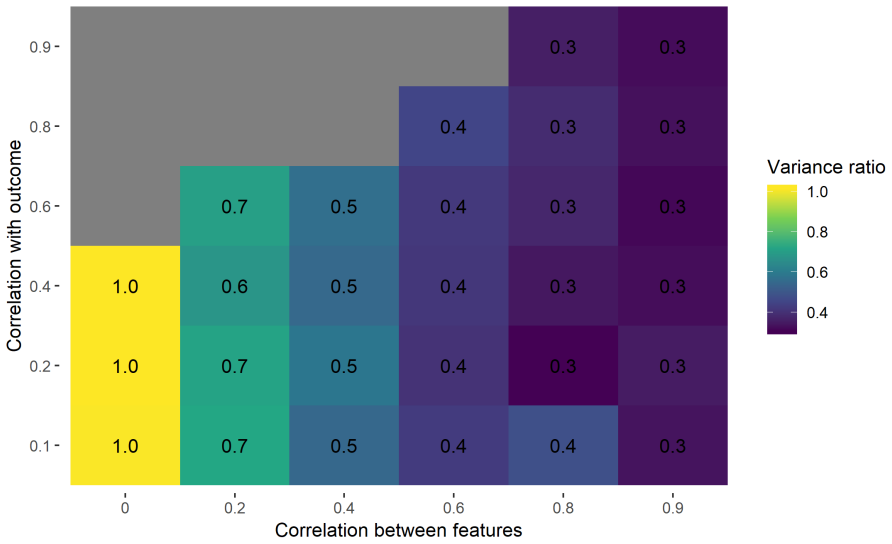
Summary. This paper proposes a global feature-importance metric for machine learning models. The method first computes a baseline R2 as var(yhat)/(var(yhat)+varres), then for each feature f constructs a modified prediction yhat_i - phi_i^f using instance-level SHAP values, and finally normalizes the resulting residual-variance ratios in Eq. (6) so that the feature-level scores sum to the baseline R2. The authors claim that this metric 'fairly allocates' model-explained variability, is bounded between 0 and 1, requires no model refitting, and can be computed from precomputed Shapley values. The paper includes a correlation-adjustment index sigma_unique (Eq. (7)), a simulation of that index, and applied demonstrations on wine quality and forest-fire datasets using CatBoost.
Significance. The practical motivation is good: a model-agnostic, refit-free global importance measure that reuses exact TreeSHAP values would be useful, and the authors provide an open-source R package. The paper also correctly identifies that LMG-type Shapley decompositions require refitting and are computationally expensive. However, the central theoretical claim is not established: Eq. (6) is a normalization of residual-variance increases, not a Shapley decomposition of R2, and the paper's fairness claim is demonstrably false under the standard Shapley/LMG notion in a simple linear model. The sigma_unique formula also contains a definite error. As submitted, the contribution is a heuristic with a misleading name rather than a rigorous decomposition.
major comments (3)
- [Proposed R2 Feature Importance Metric, Eq. (6), and Abstract] The claim that Eq. (6) is a 'Shapley-value variance decomposition' that 'fairly allocates' explained variance is not supported. The decomposition into shares that sum to R2_baseline is imposed by the normalization in the denominator of Eq. (6); no game over feature subsets is defined, and none of the Shapley axioms (efficiency, symmetry, dummy, additivity) is verified. The metric is therefore a normalized residual-variance-increase heuristic, not a Shapley decomposition. This is not a semantic quibble: in the linear model y = x1 + sqrt(3) x2 + eps with independent standard-normal x1, x2, eps, the classical Shapley/LMG shares of R2 = 0.8 are (0.2, 0.6), while Eq. (6) applied to exact SHAP values yields (0.32, 0.48). Thus the 'fair allocation' claim is false under the standard notion of Shapley fairness, even in the idealized uncorrelated case that the paper highlights.
- [Proposed R2 Feature Importance Metric, Eq. (5)] The construction yhat_i - phi_i^f is interpreted as removing feature f's marginal contribution from the prediction. This is not generally valid for nonlinear or interacting models. SHAP values are local additive attributions that depend on all features; the vector y - (yhat_i - phi_i^f) is not the prediction error of a model trained or evaluated without feature f. The variance increase after this subtraction therefore reflects covariance and interaction terms involving other features, not a quantity that can be uniquely attributed to feature f. The discussion of 'unique variance' in the correlation section consequently overstates what the metric measures.
- [Accounting for Correlation, Eq. (7)] The formula for sigma_unique is inconsistent with the definition in the text and with the claimed value of 1 for uncorrelated features. As written, the numerator is the sum of the raw residual variances after each feature is removed, not the sum of increases in residual variance. In the same two-feature example, the numerator is var(x1 + eps) + var(sqrt(3)x2 + eps) = 2 + 4 = 6, while the denominator is var(y) - var(eps) = 4, giving sigma_unique = 1.5 rather than 1. To obtain the intended quantity, each term would need to be the increase over the baseline residual variance, that is, sum_f [var(y - yhat_shap(f)) - var(y - yhat)]. As printed, Eq. (7), Figure 1, and the sigma_unique values in the applied section do not measure what is claimed.
minor comments (5)
- [Related Work] There is a typo: 'Lundburg' should be 'Lundberg'.
- [Proposed R2 Feature Importance Metric, Eq. (6)] The paper should state the edge case in which the denominator of Eq. (6) is zero, for example when R2_baseline = 0 or all raw numerators are zero.
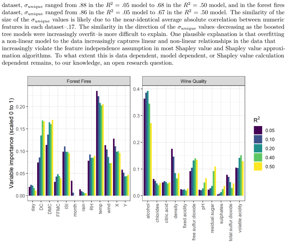
- [Applied Analysis] The applied analysis is purely descriptive: there is no comparison with LMG, permutation importance, or other global importance methods, and no uncertainty quantification for the reported rankings.
- [Applied Analysis, Figure 2] Please define the axes in Figure 2 and explain how the 0-1 scaling affects the interpretation; as drawn, the figure makes it difficult to assess changes relative to the underlying model R2.
- [Accounting for Correlation, Eq. (7)] The notation var(y - ybar) should be spelled out as var(y - mean(y)) to avoid confusion with the fitted values yhat.
Circularity Check
Sum-to-R2 property is enforced by normalization in Eq. (6), but the paper has no fitted-input or self-citation circularity.
-
self definitional
[Eq. (6), Section 'Proposed R2 Feature Importance Metric']
"The denominator of (6) normalizes the R2 values to produce a simplex similar to that produced by the softmax function. Finally, multiplying this vector of feature-level variance explained attributions with R2baseline ensures that R2baseline := sum_f R2(f)shap."
The advertised property that the feature shares sum to the overall model R2 is not derived from Shapley axioms or from the data; it is inserted by the normalization in Eq. (6). The paper presents this summation as a desirable property of the method, but it holds by construction of the formula. Thus the 'decomposition summing to the overall R2' is definitional rather than an independent finding. This is a limited circularity because the metric is a proposed definition, not a fitted quantity that is recycled as a prediction.
full rationale
The main derivation chain is self-contained: Eq. (4) defines a baseline R2, Eq. (5) defines Shapley-modified predictions, Eq. (6) defines feature shares from residual-variance ratios, and Eq. (7) defines a uniqueness ratio. No parameter is fitted to a subset of the data and later renamed as a prediction, and no external benchmark is predicted from fitted constants. The wine and forest-fires analyses are illustrative demonstrations of stability rather than tests that could falsify the sum-to-R2 property. There are no load-bearing self-citations: the author's own shapFlex package appears only as an implementation link, while the Shapley additivity and LMG results are cited from independent literature. The one definitional circularity is the sum property, which Eq. (6) enforces by normalization; the broader 'fair allocation' claim is an interpretive choice about what the normalized residual-variance changes mean, not a circular derivation. Score 2 reflects this single self-definitional property while recognizing that the central construction is otherwise independent of its inputs.
Assumptions & free parameters
assumptions (3)
- domain assumption For a fitted model, Shapley values are additive: yhat_i = phi_0 + sum_f phi_i^f (Eq. 3), so subtracting phi_i^f removes feature f from the prediction.
- domain assumption An increase in residual variance after subtracting a feature's Shapley values measures that feature's unique explained variance (Eq. 7).
- domain assumption TreeSHAP values used in the applied analysis are treated as exact and reliable Shapley values.
Cite this review
Pith. "Pith review of Shapley Decomposition of R-Squared in Machine Learning Models." pith.science (2026). https://pith.science/paper/NRYEU3DM
@misc{pith2026190809718,
  author       = {Pith},
  title        = {Pith review of: Shapley Decomposition of R-Squared in Machine Learning Models},
  year         = {2026},
  howpublished = {\url{https://pith.science/paper/NRYEU3DM}},
  note         = {Machine review of arXiv:1908.09718}
}
abstract
In this paper we introduce a metric aimed at helping machine learning practitioners quickly summarize and communicate the overall importance of each feature in any black-box machine learning prediction model. Our proposed metric, based on a Shapley-value variance decomposition of the familiar $R^2$ from classical statistics, is a model-agnostic approach for assessing feature importance that fairly allocates the proportion of model-explained variability in the data to each model feature. This metric has several desirable properties including boundedness at 0 and 1 and a feature-level variance decomposition summing to the overall model $R^2$. In contrast to related methods for computing feature-level $R^2$ variance decompositions with linear models, our method makes use of pre-computed Shapley values which effectively shifts the computational burden from iteratively fitting many models to the Shapley values themselves. And with recent advancements in Shapley value calculations for gradient boosted decision trees and neural networks, computing our proposed metric after model training can come with minimal computational overhead. Our implementation is available in the R package shapFlex.
Figures
Reference graph
Works this paper leans on
-
[1]
J., Singh, C., Kumbier, K., Abbasi-Asl, R., & Yu, B
Murdoch, W. J., Singh, C., Kumbier, K., Abbasi-Asl, R., & Yu, B. (2019). Interpretable machine learning: definitions, methods, and applications. arXiv preprint arXiv:1901.04592
arXiv 2019
-
[2]
Doshi-Velez, F., & Kim, B. (2017). Towards a rigorous science of interpretable machine learning. arXiv preprint arXiv:1702.08608
arXiv 2017
-
[3]
Lundberg, S. M., & Lee, S. I. (2017). A unified approach to interpreting model predictions. In Advances in Neural Information Processing Systems (pp. 4765-4774)
work page 2017
-
[4]
Biecek, P. (2018). DALEX: explainers for complex predictive models in R. The Journal of Machine Learning Research, 19(1), 3245-3249
work page 2018
-
[5]
Molnar, C., Casalicchio, G., & Bischl, B. (2018). Iml: An R package for interpretable machine learning. The Journal of Open Source Software, 3(786), 10-21105
work page 2018
-
[6]
Interpretable machine learning. A Guide for Making Black Box Models Explainable
Molnar, Christoph. (2019) “Interpretable machine learning. A Guide for Making Black Box Models Explainable”. https://christophm.github.io/interpretable-ml-book/
work page 2019
-
[7]
Britton, M. (2019). VINE: Visualizing Statistical Interactions in Black Box Models. arXiv preprint arXiv:1904.00561
work page Pith review arXiv 2019
-
[8]
Grömping, U. (2015). Variable importance in regression models. Wiley Interdisciplinary Reviews: Computational Statistics, 7(2), 137-152
work page 2015
Show all 22 references
-
[9]
Wachter, S., Mittelstadt, B., & Russell, C. (2017). Counterfactual explanations without opening the black box: Automated decisions and the GDPR. Harvard Journal of Law & Technology, 31(2), 2018
2017
-
[10]
Wright, S. (1921). Correlation and causation. Journal of agricultural research, 20(7), 557-585
1921
-
[11]
Kvålseth, T. O. (1985). Cautionary note about R 2. The American Statistician, 39(4), 279-285
1985
-
[12]
Fisher, A., Rudin, C., & Dominici, F. (2018). All Models are Wrong but many are Useful: Variable Importance for Black-Box, Proprietary, or Misspecified Prediction Models, using Model Class Reliance. arXiv preprint arXiv:1801.01489
2018 arXiv
-
[13]
Gelman, A., Goodrich, B., Gabry, J., & Vehtari, A. (2018). R-squared for Bayesian regression models. The American Statistician, (just-accepted), 1-6
2018
-
[14]
Lideman, R., Merenda, P., & Gold, R. (1980). Introduction to bivariate and multivariate analysis scott. Scott Foresman: Glenview, IL, USA
1980
-
[15]
D., (2017) Decomposing the R-squared of a Regression Using the Shapley Value in SAS®
Coleman, C. D., (2017) Decomposing the R-squared of a Regression Using the Shapley Value in SAS®. US Census Bureau
2017
-
[16]
Shapley, L. S. (1953). A value for n-person games. In Kuhn, H. W. and Tucker, A. W., editors, Contribution to the Theory of Games II (Annals of Mathematics Studies 28), pages 307–317. Princeton University Press, Princeton, NJ
1953
-
[17]
M., Erion, G
Lundberg, S. M., Erion, G. G., & Lee, S. I. (2018). Consistent individualized feature attribution for tree ensembles. arXiv preprint arXiv:1802.03888
2018 arXiv
-
[18]
Explaining individual predictions when features are dependent: More accurate approximations to Shapley values
Kjersti, Aas, Jullum, Martin, & Løland, Anders (2019). Explaining individual predictions when features are dependent: More accurate approximations to Shapley values. arXiv preprint arXiv:1903.10464v2
2019 arXiv
-
[19]
Cortez, A
P. Cortez, A. Cerdeira, F. Almeida, T. Matos and J. Reis. (2009). Modeling wine preferences by data mining from physicochemical properties. In Decision Support Systems, Elsevier, 47(4):547-553. 8
2009
-
[20]
Cortez & A
P. Cortez & A. Morais. (2007). A Data Mining Approach to Predict Forest Fires using Meteorological Data. In J. Neves, M. F. Santos and J. Machado Eds., New Trends in Artificial Intelligence, Proceedings of the 13th EPIA 2007 - Portuguese Conference on Artificial Intelligence, De...
2007
-
[21]
& Graff, C
Dua, D. & Graff, C. (2019). UCI Machine Learning Repository [http://archive.ics.uci.edu/ml]. Irvine, CA: University of California, School of Information and Computer Science
2019
-
[22]
V., & Gulin, A
Prokhorenkova, L., Gusev, G., Vorobev, A., Dorogush, A. V., & Gulin, A. (2018). CatBoost: unbiased boosting with categorical features. In Advances in Neural Information Processing Systems (pp. 6638- 6648). 9
2018
Reviewed August 14, 2026 · model on record in the stance chip above.
Discussion (0). Continue with ORCID to comment.