REVIEW 3 major objections 5 minor 44 references
A statistical framework for measuring the temporal stability of human mobility patterns
T0 review · 3 major / 5 minor · reviewed 2026-08-14 · deepseek-v4-flash
Pith's one-line read The paper claims that GPS monitoring must last at least 15 weeks—roughly seven times the current 14-day recommendation—to capture temporally stable human mobility patterns, with average stabilization times of 30 weeks for velocity and 37…
desk verdict New stability measures for GPS mobility are worth knowing, but the 'at least 15 weeks' headline is not backed by the paper's own tables and the LCT approach needs a stability check before its durations are used. read the letter →
The pith
A machine-rendered reading of the paper's core claim, the machinery that carries it, and where it could break.
The reading
What carries the argument
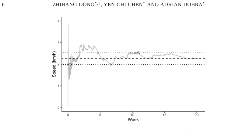
The engine is the last crossing time (LCT) process. For a process $Z(\tau)$ summarizing the trajectory up to time $\tau$—average velocity or the estimated weekly activity distribution—the LCT is the largest $\tau$ at which the absolute percentage error $\varphi(Z;\tau) = |Z(\tau) - Z(T)|/Z(T)$ still exceeds a threshold $\gamma$; it says how long one must observe before the prefix estimate stops disagreeing with the full-record estimate. The supporting machinery includes two estimators of the distribution of time spent in spatial grid cells, the ordinary and conservative proportional time estimators, which the paper proves are asymptotically equivalent and consistent, and a ranking-based $\alpha$-level set that focuses the stability check on the grid cells where a person actually spends most of their time.
What would settle it
Recompute the three last-crossing-time measures on a GPS panel that runs three years or more; if median LCT-velocity rises above 30 weeks or a large share of participants still have last crossing times at the end of the observation window, the paper's stabilization times are censored by the 18-month horizon.
Extended reading notes
Core claim
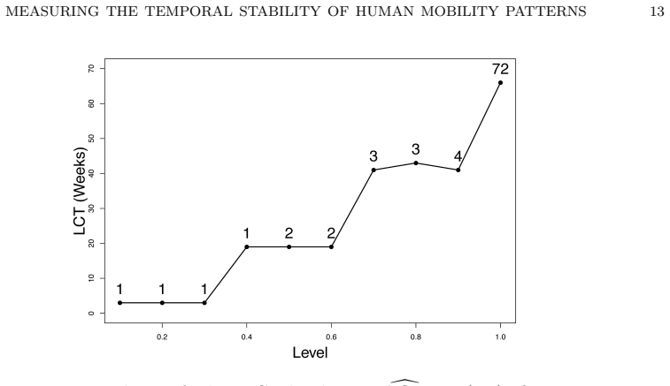
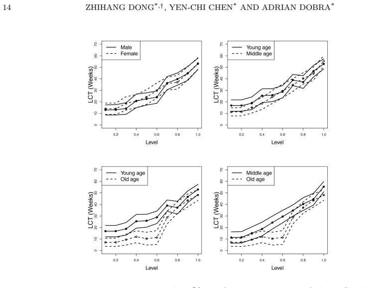
The central claim is that human mobility patterns, as recorded by GPS, take far longer to become temporally stable than previous empirical work suggested. Using the last crossing time of the absolute percentage error with threshold $\gamma = 0.2$, the authors find mean stabilization times of 30.04 weeks for average velocity, 37.18 weeks for the weekly activity distribution, and 17.69 weeks for the 0.2-level set of important places, and conclude that GPS monitoring needs to last at least 15 weeks—about seven times the 14 days recommended by the earlier study. A second claim is that stability is demographic: older adults' mobility stabilizes sooner (about 10 weeks for the level-set measure), middle-aged adults need about 15 weeks, and younger adults about 20 weeks, so study designs should set durations by demographic group rather than a single universal window.
Load-bearing premise
The load-bearing premise is that the estimate computed from the entire 18-month window equals each person's stable long-run mobility pattern; if the window is too short, every reported minimum duration is a lower bound rather than a true stabilization time.
Editorial extensions
If this is right
- Seven- to fourteen-day GPS studies, common in health and social research, are likely to record mobility patterns that are still changing; conclusions drawn from them may not reflect stable long-run behavior.
- A minimum monitoring length of about 15 weeks is needed for stable estimates; studies targeting full weekly activity distributions should plan for roughly 37 weeks, while studies that only need the main places of activity can use about 18 weeks.
- Differential study durations by demographic group are warranted: older adults stabilize faster, so shorter monitoring may suffice, while younger adults need longer windows.
- The ordinary and conservative proportional time estimators give consistent recovery of activity distributions even when GPS sampling is irregular, so researchers can use them to correct for non-uniform observation times.
- The level-set measure provides a way to separate stability of core places from stability of rarely visited places, so researchers can tailor the observation window to the spatial resolution their research question needs.
Reading between the lines
- Because every LCT is measured against the estimate from the entire 18-month window, the quoted stabilization times are best read as lower bounds tied to that window; a longer observation study could push them upward if truly stable patterns emerge only after more than 18 months.
- The same last-crossing-time template could be applied to other longitudinal behavioral records (e.g., daily retail visits, app usage, or mobility from call detail records) by replacing the velocity or activity distribution process with the relevant summary statistic.
- The demographic pattern suggests an adaptive design in which monitoring continues until a participant-specific LCT drops below a threshold, which could reduce participant burden while preserving stability guarantees.
- Because the consistency theorems assume increasingly dense sampling, a testable implication is that much denser GPS recording could shorten the required calendar duration to reach the same stability level.
Signed reviews
Editorial analysis
A structured set of objections, weighed in public.
Referee Report
Summary. The paper proposes a statistical framework for determining the minimum required length of GPS monitoring for human mobility studies. It defines last-crossing-time (LCT) measures based on the average velocity process and on activity distributions over a spatial grid, introduces ordinary and conservative proportional time estimators for activity distributions, and proves their asymptotic equivalence and consistency under assumptions (S1)-(S3). The method is applied to the Nokia Mobile Data Challenge, with GPS data from 185 individuals over about 18 months. The empirical results give mean LCT values of roughly 30 weeks for velocity, 37 weeks for the full activity distribution, and 18 weeks for the 0.2-level set of important places. The authors conclude that GPS monitoring should last at least 15 weeks, about seven times longer than the 14-day recommendation of Zenk et al., and that study duration should depend on demographic group.
Significance. If the empirical claims held, the paper would provide a valuable theoretical basis for a design question that has so far been addressed mainly empirically: how long GPS monitoring must last. The theoretical results are a genuine contribution: the consistency and asymptotic equivalence proofs for the proportional time estimators are clean under assumptions (S1)-(S3), and the LCT formalism gives a concrete, interpretable target for stabilization. The paper also makes constructive use of a publicly available longitudinal GPS dataset and makes falsifiable quantitative predictions (e.g., 30, 37, and 18 weeks in Table 1). However, the central empirical conclusion depends on an assumption about the endpoint of the observation window that is not tested, and the headline 'at least 15 weeks' is not directly supported by the table of aggregate results. The framework is promising, but the central design recommendation needs substantially more validation before it can be accepted.
major comments (3)
- [Sections 2.1 and 2.3, Eqs. (6), (14), and (17)] All three LCT measures are defined relative to the final value of the process over the entire observed window: Eq. (6) uses Z(tmax-tmin), Eq. (14) uses \hat{\bar{\pi}}(Dmax), and Eq. (17) uses Lα(Dmax). These are retrospective summaries of the particular 18-month MDC window, not estimates of a stable long-run mobility pattern. The paper's design recommendation assumes that the final estimate is close to each individual's stable mobility pattern, but it provides no check of this assumption: there is no split-half validation, no holdout-period comparison, no assessment of drift or nonstationarity over the study period, and no report of how many participants' LCTs are censored at the horizon. Without such checks, a short LCT can occur simply because the endpoint itself has moved, and a long LCT for a genuinely unstable individual may be truncated at Dmax. The 'minimum required length' conclusion is therefore contaminated by the arbitrary length of the observation window unless endpoint stability is established.
- [Section 3, Table 1, and Section 4, Discussion] The aggregate results in Table 1 report mean LCTs of 30.04 weeks (velocity), 37.18 weeks (distribution), and 17.69 weeks (0.2-level set), yet the Discussion concludes that GPS monitoring needs to be done for 'at least 15 weeks.' This number does not follow from Table 1: it is closer to the subgroup-specific value for middle-age participants shown in Figure 4 for the level-set measure, and it is far below the mean for the other two measures. A minimum study duration should be derived from an explicit design criterion, typically an upper quantile of the distribution across participants, not from subgroup means. The paper should reconcile Table 1 with the Discussion, report the quantiles of the LCT distributions, and state how much censoring occurs at Dmax.
- [Section 3, Figure 4] The claim that study duration should differ by demographic group is based on visual comparison of mean LCT curves with 90% confidence intervals. No formal test, effect size, or adjustment for repeated measures or multiple comparisons is provided, and the confidence intervals are not defined (standard error? bootstrap? adjusted for within-person correlation?). Since demographic differentiation is presented as a second substantive contribution, it needs supporting inference rather than descriptive curves alone.
minor comments (5)
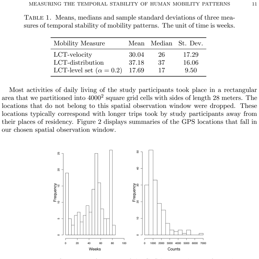
- [Section 3, first paragraph of Application] The text says the window is partitioned into '40002 square grid cells' while later text uses N = 4000^2; 4000^2 is 16,000,000, not 4,000. Please clarify the grid resolution and the total number of cells.
- [Section 2.3, text before Eq. (13)] The sentence 'We denote by π(d) the activity distribution from Eq. (12) associated with time period D' conflates the true activity distribution from Eq. (9) with the estimator from Eq. (12). Please separate the estimand from the estimator.
- [Section 2.3, Eq. (17)] The denominator ||Lα(Dmax)|| can be zero for some participants or some values of α; please state a convention (e.g., define the LCT as 0 in that case) so that the ratio is well defined.
- [Section 2.1, Eq. (5)] The estimator \hat V_k(τ) sums distances between consecutive observation times with t_{k,i+1} ≤ τ, which omits the partial segment between the last recorded time before τ and τ itself; please state this explicitly or use interpolation.
- [Figure 2 caption] There is a typo: 'histrogram' should be 'histogram'.
Circularity Check
No significant circularity: the LCT measures are well-defined statistics, and the endpoint dependence is a validity limitation rather than a circular derivation.
full rationale
The paper's derivation chain is self-contained. The last-crossing-time measures in Eqs. (6), (14), and (17) are explicitly defined statistics of the observed trajectory, and the empirical values in Table 1 and Figure 4 are computed from the MDC data rather than fitted to reproduce a target conclusion. Theorems 2.1 and 2.2 are proved directly in Appendix A under the stated sampling assumptions (S1)-(S3), so the consistency results do not rely on self-citation or on the empirical claim. The only structural concern is that LCT is defined relative to the final value over the observation window, e.g., Z(tmax-tmin) in Eq. (6) and \hat{\bar{\pi}}(Dmax) in Eq. (14), so the reported stabilization times are contingent on the 18-month horizon; if the endpoint is not the individual's stable long-run pattern, the recommended 'at least 15 weeks' is a lower bound. That is a substantive validity/identifiability limitation, not a circular reduction: no equation reduces to its own input, no fitted parameter is renamed as a prediction, and the central claim is not forced by a self-citation chain. The citation to the authors' prior work [7] for the ranking distribution in Eq. (15) is definitional and not load-bearing. Therefore no significant circularity is present.
Assumptions & free parameters
free parameters (4)
- stability threshold gamma =
0.2
- level set parameter alpha =
0.2
- grid cell side length =
28 meters
- spatial observation window =
rectangular area excluding longer trips
assumptions (5)
- domain assumption The spatiotemporal trajectory is smooth, with continuous derivatives for x1 and x2 (Eq. 1).
- domain assumption T follows a uniform distribution on [tmin, tmax] in the definition of the activity distribution (Eq. 9).
- domain assumption Assumptions (S1)-(S3): dense observation times, boundary coverage, and finite grid transitions.
- domain assumption Study participants traveled in a straight line between consecutive observed GPS locations.
- domain assumption The grid-cell mapping and proportional-time estimators recover time spent in cells, with transition intervals handled by the ordinary or conservative estimators.
Cite this review
Pith. "Pith review of A statistical framework for measuring the temporal stability of human mobility patterns." pith.science (2026). https://pith.science/paper/5TJIIJYN
@misc{pith2026190809830,
  author       = {Pith},
  title        = {Pith review of: A statistical framework for measuring the temporal stability of human mobility patterns},
  year         = {2026},
  howpublished = {\url{https://pith.science/paper/5TJIIJYN}},
  note         = {Machine review of arXiv:1908.09830}
}
read the original abstract
Despite the growing popularity of human mobility studies that collect GPS location data, the problem of determining the minimum required length of GPS monitoring has not been addressed in the current statistical literature. In this paper we tackle this problem by laying out a theoretical framework for assessing the temporal stability of human mobility based on GPS location data. We define several measures of the temporal dynamics of human spatiotemporal trajectories based on the average velocity process, and on activity distributions in a spatial observation window. We demonstrate the use of our methods with data that comprise the GPS locations of 185 individuals over the course of 18 months. Our empirical results suggest that GPS monitoring should be performed over periods of time that are significantly longer than what has been previously suggested. Furthermore, we argue that GPS study designs should take into account demographic groups. KEYWORDS: Density estimation; global positioning systems (GPS); human mobility; spatiotemporal trajectories; temporal dynamics
Figures
Figures from the paper (2 more)
Reference graph
Works this paper leans on
-
[1]
L.A. Basta, T.S. Richmond, and D.J. Wiebe, Neighborhoods, daily activities, and measuring health risks experienced in urban environments , Social Science & Medicine 71 (2010), pp. 1943–1950
work page 2010
-
[2]
J. Beekhuizen, H. Kromhout, A. Huss, and R. Vermeulen, Performance of GPS-devices for envi- ronmental exposure assessment, Journal of Exposure Science and Environmental Epidemiology 23 (2013), pp. 498–505
work page 2013
-
[3]
D. Berrigan, J.A. Hipp, P.M. Hurvitz, P. James, M.M. Jankowska, J. Kerr, F. Laden, T. Leonard, R.A. McKinnon, T.M. Powell-Wiley, E. Tarlov, S.N. Zenk, and The TREC Spatial and Contextual, Measures and Modeling Work Group, Geospatial and contextual approaches to energy balance and health, Annals of GIS 21 (2015), pp. 157–168. 18 ZHIHANG DONG *,†, YEN-CHI C...
work page 2015
- [4]
-
[5]
C.R. Browning, C.A. Calder, B. Soller, A.L. Jackson, and J. Dirlam, Ecological networks and neigh- borhood social organization, American Journal of Sociology 122 (2017), pp. 1939–1988
work page 2017
-
[6]
H. Byrnes, B.A. Miller, C.N. Morrison, D.J. Wiebe, M. Woychik, and S.E. Wiehe, Association of environmental indicators with teen alcohol use and problem behavior: Teens’ observations vs. objectively-measured indicators, Health & Place 43 (2017), pp. 151–157
work page 2017
-
[7]
Chen, Generalized cluster trees and singular measures , Annals of Statistics 47 (2019), pp
Y.C. Chen, Generalized cluster trees and singular measures , Annals of Statistics 47 (2019), pp. 2174–2203
work page 2019
-
[8]
W.J. Christian, Using geospatial technologies to explore activity-based retail food environments, Spa- tial and Spatio-temporal Epidemiology 3 (2012), pp. 287–295
work page 2012
Show all 44 references
-
[9]
Courant and F
R. Courant and F. John, Introduction to Calculus and Analysis , Vol. I, Springer, New York, 1991
1991
-
[10]
Dobra and N.E
A. Dobra and N.E. Williams, Spatiotemporal detection of unusual human population behavior using mobile phone data , PLoS ONE 10 (2015), p. e0120449
2015
-
[11]
Duncan, D.A
D.T. Duncan, D.A. Hickson, W.C. Goedel, D. Callander, B. Brooks, Y.T. Chen, H. Hanson, R. Eavou, A.S. Khanna, B. Chaix, S. Regan, D.P. Wheeler, K.H. Mayer, S.A. Safren, M.S. Carr, C. Draper, V. Magee-Jackson, R. Brewer, and J.A. Schneider, International Journal of Environmenta...
2019
-
[12]
Duncan, F
D.T. Duncan, F. Kapadia, S.D. Regan, W.C. Goedel, M.D. Levy, S.C. Barton, S.R. Friedman, and P.N. Halkitis, Feasibility and acceptability of Global Positioning System (GPS) methods to study the spatial contexts of substance use and sexual risk behaviors among young men who hav...
2016
-
[13]
Elgethun, M.G
K. Elgethun, M.G. Yost, C.T. Fitzpatrick, T.L. Nyerges, and R.A. Fenske, Comparison of Global Positioning System (GPS) tracking and parent-report diaries to characterize children’s time-location patterns, Journal of Exposure Science and Environmental Epidemiology 17 (2007), pp...
2007
-
[14]
Entwisle, Putting people into place , Demography 44 (2007), pp
B. Entwisle, Putting people into place , Demography 44 (2007), pp. 687–703
2007
-
[15]
Graif, A.S
C. Graif, A.S. Gladfelter, and S.A. Matthews, Urban poverty and neighborhood effects on crime: Incorporating spatial and network perspectives, Sociology Compass 8 (2014), pp. 1140–1155
2014
-
[16]
Harding, Z
C. Harding, Z. Patterson, L. Miranda-Moreno, and S. Zahabi, Modeling the effect of land use on activity spaces, Transportation Research Record: Journal of the Transportation Research Board 2323 (2012), pp. 67–74
2012
-
[17]
Kestens, A
Y. Kestens, A. Lebel, M. Daniel, M. Th´ eriault, and R. Pampalon,Using experienced activity spaces to measure foodscape exposure, Health & Place 16 (2010), pp. 1094–1103
2010
-
[18]
Kiukkonen, J
N. Kiukkonen, J. Blom, O. Dousse, D. Gatica-Perez, and J. Laurila, Towards Rich Mobile Phone Datasets: Lausanne Data Collection Campaign , in Proc. ACM Int. Conf. on Pervasive Services (ICPS), Berlin, July. 2010
2010
-
[19]
Kopec, Concepts of disability: The activity space model , Social Science & Medicine 40 (1996), pp
J.A. Kopec, Concepts of disability: The activity space model , Social Science & Medicine 40 (1996), pp. 649–656
1996
-
[20]
Krivo, H.M
L.J. Krivo, H.M. Washington, R.D. Peterson, C.R. Browning, C.A. Calder, and M.P. Kwan, Social isolation of disadvantage and advantage: The reproduction of inequality in urban space, Social Forces 92 (2013), pp. 141–164
2013
-
[21]
Kwan, The uncertain geographic context problem , Annals of the Association of American Geographers 102 (2012), pp
M.P. Kwan, The uncertain geographic context problem , Annals of the Association of American Geographers 102 (2012), pp. 958–968
2012
-
[22]
M.P. Kwan, Beyond space (as we knew it): Toward temporally integrated geographies of segregation, health, and accessibility, Annals of the Association of American Geographers 103 (2013), pp. 1078– 1086
2013
-
[23]
Laurila, D
J.K. Laurila, D. Gatica-Perez, I. Aad, J. Blom, O. Bornet, T. Do, O. Dousse, J. Eberle, and M. Miettinen, The Mobile Data Challenge: Big Data for Mobile Computing Research , in Proc. Mobile Data Challenge Workshop (MDC) in conjunction with Int. Conf. on Pervasive Computing, Ne...
2012
-
[24]
Laurila, D
J.K. Laurila, D. Gatica-Perez, I. Aad, J. Blom, O. Bornet, T.M.T. Do, O. Dousse, J. Eberle, and M. Miettinen, From big smartphone data to worldwide research: The Mobile Data Challenge , Pervasive and Mobile Computing 9 (2013), pp. 752–771. MEASURING THE TEMPORAL STABILITY OF H...
2013
-
[25]
Lee, A.W
J.H. Lee, A.W. Davis, S.Y. Yoon, and K.G. Goulias, Activity space estimation with longitudinal observations of social media data , Transportation 43 (2016), pp. 955–977
2016
-
[26]
Matthews and T.C
S.A. Matthews and T.C. Yang, Spatial polygamy and contextual exposures (SPACEs): Promoting activity space approaches in research on place and health. , The American Behavioral Scientist 57 (2013), pp. 1057–1081
2013
-
[27]
Mazimpaka and S
J.D. Mazimpaka and S. Timpf, Trajectory data mining: A review of methods and applications , Journal of Spatial Information Science 13 (2016), pp. 61–99
2016
-
[28]
Miller, Place-based versus people-based Geographic Information Science , Geography Compass 1 (2007), pp
H. Miller, Place-based versus people-based Geographic Information Science , Geography Compass 1 (2007), pp. 503–535
2007
-
[29]
Morrison, H.F
C.N. Morrison, H.F. Byrnes, B.A. Miller, E. Kaner, S.E. Wiehe, W.R. Ponicki, and D. Wiebe, Assessing individuals’ exposure to environmental conditions using residence-based measures, activity location-based measures, and activity path-based measures, Epidemiology 30 (2019), pp...
2019
-
[30]
Newsome, W.A
T.H. Newsome, W.A. Walcott, and P.D. Smith, Urban activity spaces: Illustrations and application of a conceptual model for integrating the time and space dimensions , Transportation 25 (1998), pp. 357–377
1998
-
[31]
Noah, Putting families into place: Using neighborhood-effects research and activity spaces to understand families, Journal of Family Theory & Review 7 (2015), pp
A.J. Noah, Putting families into place: Using neighborhood-effects research and activity spaces to understand families, Journal of Family Theory & Review 7 (2015), pp. 452–467
2015
-
[32]
Paul, Female activity space in rural Bangladesh , Geographical Review 82 (1992), pp
B.K. Paul, Female activity space in rural Bangladesh , Geographical Review 82 (1992), pp. 1–12
1992
-
[33]
Perchoux, B
C. Perchoux, B. Chaix, S. Cummins, and Y. Kestens, Conceptualization and measurement of envi- ronmental exposure in epidemiology: Accounting for activity space related to daily mobility , Health & Place 21 (2013), pp. 86–93
2013
-
[34]
Richardson, N.D
D.B. Richardson, N.D. Volkow, M.P. Kwan, R.M. Kaplan, M.F. Goodchild, and R.T. Croyle,Spatial turn in health research, Science 339 (2013), pp. 1390–1392
2013
-
[35]
Schonfelder and K.W
S. Schonfelder and K.W. Axhausen, Activity spaces: Measures of social exclusion?, Transport Policy 10 (2003), pp. 273–286
2003
-
[36]
Sherman, J
J.E. Sherman, J. Spencer, J.S. Preisser, W.M. Gesler, and T.A. Arcury, A suite of methods for repre- senting activity space in a healthcare accessibility study, International Journal of Health Geographics 4 (2015), p. 24
2015
-
[37]
VanWey, R.R
L.K. VanWey, R.R. Rindfuss, M.P. Gutmann, B. Entwisle, and D.L. Balk, Confidentiality and spatially explicit data: Concerns and challenges , Proceedings of the National Academy of Sciences 102 (2005), pp. 15337–15342
2005
-
[38]
Vazquez-Prokopec, D
G.M. Vazquez-Prokopec, D. Bisanzio, S.T. Stoddard, V. Paz-Soldan, A.C. Morrison, J.P. Elder, J. Ramirez-Paredes, E.S. Halsey, T.J. Kochel, and T.W. Scott, Using GPS technology to quan- tify human mobility, dynamic contacts and infectious disease dynamics in a resource-poor urb...
2013
-
[39]
Waller and C.A
L.A. Waller and C.A. Gotway, Applied Spatial Statistics for Public Health Data , John Wiley & Sons, Hoboken, NJ, 2004
2004
-
[40]
Wasserman, All of Nonparametric Statistics , Springer Texts in Statistics, Springer, New York, 2007
L. Wasserman, All of Nonparametric Statistics , Springer Texts in Statistics, Springer, New York, 2007
2007
-
[41]
Wiehe, M.P
S.E. Wiehe, M.P. Kwan, J. Wilson, and J.D. Fortenberry, Adolescent health-risk behavior and com- munity disorder, PloS One 8 (2013), p. e77667
2013
-
[42]
Wiehe, A.E
S.E. Wiehe, A.E. Carroll, G.C. Liu, K.L. Haberkorn, S.C. Hoch, J.S. Wilson, and J.D. Fortenberry, Using gps-enabled cell phones to track the travel patterns of adolescents , International Journal of Health Geographics 7 (2008), pp. 22–22
2008
-
[43]
Zenk, S.A
S.N. Zenk, S.A. Matthews, A.N. Kraft, and K.K. Jones, How many days of Global Positioning System (GPS) monitoring do you need to measure activity space environments in health research? , Health & Place 51 (2018), pp. 52–60
2018
-
[44]
Zenk, A.J
S.N. Zenk, A.J. Schulz, S.A. Matthews, A. Odoms-Young, J. Wilbur, L. Wegrzyn, K. Gibbs, C. Braunschweig, and C. Stokes,Activity space environment and dietary and physical activity behaviors: a pilot study , Health & Place 17 (2011), pp. 1150–1161. * Department of Statistics, U...
2011
Reviewed August 14, 2026 · model on record in the stance chip above.
Discussion (0). Continue with ORCID to comment.