REVIEW 5 major objections 6 minor 74 references
Machine-assisted Semi-Simulation Model (MSSM): Estimating Galactic Baryonic Properties from their Dark Matter using a Machine Trained on Hydrodynamic Simulations
T0 review · 5 major / 6 minor · reviewed 2026-08-14 · deepseek-v4-flash
Pith's one-line read A machine trained on a hydrodynamic simulation can estimate baryonic galaxy properties from dark-matter halo properties alone, then paint them onto a gigaparsec dark-matter-only volume.
desk verdict Solid, honest engineering paper that improves ML-based halo painting with real technical contributions; the Gpc application is the weak link because the cross-simulation transfer is asserted rather than validated. read the letter →
The pith
A machine-rendered reading of the paper's core claim, the machinery that carries it, and where it could break.
The reading
What carries the argument
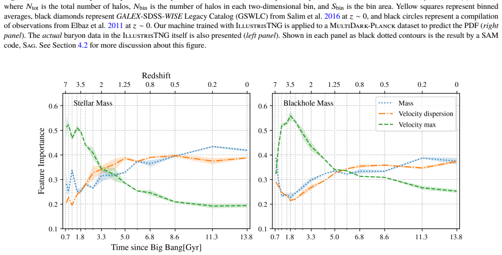
The load-bearing mechanism is the extremely randomized tree (ERT), an ensemble of decision trees that chooses node splits randomly. Three training choices carry the accuracy gain: (1) a logarithmically scaled error function, so that fractional errors at the low-mass end are not overwhelmed by absolute errors at the high-mass end; (2) additional input features extracted from each halo's merger tree and local environment, such as merger counts, last-major-merger mass ratio, local density, and the semi-potential $\Phi_s=\sum_i M_i/R_i$ within a $(2\,\mathrm{Mpc})^3$ volume; and (3) two-stage learning, in which a first ERT predicts stellar magnitudes from dark-matter features and those predicted magnitudes become inputs to a second ERT that predicts star formation rate. The first machine also outputs feature importances, which show maximum circular velocity dominating at high redshift and halo mass and velocity dispersion taking over by $z=0$.
What would settle it
Run the trained MSSM on IllustrisTNG-Dark, the dark-matter-only counterpart of the training simulation, and compare predicted stellar masses with the actual stellar masses of matched halos in the hydrodynamic run: a systematic bias in the $M_\star$-$M_{\mathrm{halo}}$ relation, or a scatter larger than the intrinsic scatter of that relation, would falsify the transferability assumption. A second check is to compare the two-point galaxy clustering of the MDPL2 catalogue with observed clustering at fixed stellar mass; a significant mismatch would show that the machine's galaxy-halo connection is not faithful enough for large-volume statistics.
Extended reading notes
Core claim
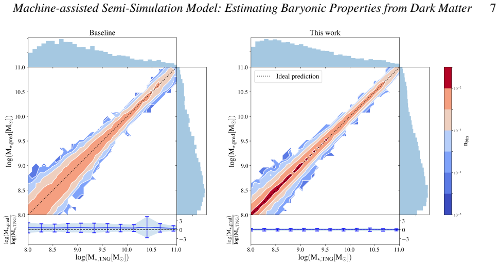
The paper's central claim is that the baryonic content of a galaxy is predictable, to useful accuracy, from the bulk properties of its dark-matter halo alone, once a machine has been shown enough examples from a hydrodynamic simulation. In the reported test, stellar mass prediction improves from a mean binned error of $0.0018$ (baseline) to $0.0013$, and star formation rate from $1.71$ to $1.00$; the predicted probability distributions for all six baryonic properties move closer to the IllustrisTNG data. When the trained machine is applied to the MultiDark-Planck dark-matter-only simulation, the resulting catalogue's distribution functions are largely compatible with the SAG semi-analytic model, and for black hole mass, star formation rate, and stellar magnitudes it tracks IllustrisTNG more closely than SAG does, which is exactly the behaviour the model was designed for.
Load-bearing premise
The load-bearing premise is that halos in a dark-matter-only simulation match halos in the hydrodynamic simulation closely enough for the learned galaxy-halo mapping to carry over, and that the two simulations' halo mass definitions are compatible after the mass cut; the paper's support for this is a less than 1% agreement in the overall halo mass function, not per-halo comparisons.
Editorial extensions
If this is right
- Large-scale galaxy catalogues from dark-matter-only runs become a matter of minutes: the machine paints roughly $10^6$ halos in a $(1\,h^{-1}\,\mathrm{Gpc})^3$ volume in tens of minutes, versus weeks for a hydrodynamic simulation.
- The baryon physics of a specific hydrodynamic simulation can be transplanted onto any sufficiently resolved dark-matter-only simulation without analytic recipes or tuned parameters.
- Differences between MSSM and SAM catalogues localise where SAM prescriptions deviate from hydrodynamic simulations, pointing to specific subgrid physics to improve.
- Because the machine reproduces the IllustrisTNG number densities, the resulting catalogue is suited for volume-limited studies such as baryonic acoustic oscillations and large-scale structure statistics.
Reading between the lines
- Pith inference: the two-stage learning trick should generalise; any baryonic property that is accurately predictable from dark matter and strongly correlated with a harder target could be chained as an intermediary, suggesting a searchable design space for future pipelines of this kind.
- Pith inference: because the transferability assumption is only tested on the halo mass function, a natural next experiment is to run the trained machine on IllustrisTNG-Dark and compare per-halo predictions with the hydrodynamic run; this would isolate transfer error from model error.
- Pith inference: if the machine's galaxy-halo connection is faithful, the MDPL2 catalogue could be forward-modelled into galaxy clustering, weak-lensing, or CMB-lensing predictions; discrepancies with observations would point to where IllustrisTNG's baryon physics needs revision.
- Pith inference: the feature-importance analysis suggests that at low redshift halo mass and velocity dispersion carry most of the information; adding merger-orbit or tidal features could broaden the output diversity that the paper identifies as too narrow.
Signed reviews
Editorial analysis
A structured set of objections, weighed in public.
Referee Report
Summary. The paper introduces a machine-learning pipeline, MSSM, that uses extremely randomized trees trained on the IllustrisTNG hydrodynamic simulation to predict galaxy baryonic properties (gas mass, stellar mass, black hole mass, star formation rate, metallicity, and stellar magnitudes) from dark-matter halo features. The authors propose three improvements over a baseline model: logarithmic scaling of the error function, addition of historical and environmental halo features, and a two-stage learning scheme that uses predicted stellar magnitudes as an intermediary to predict SFR or stellar mass. They report substantial accuracy gains on a held-out TNG test set, then apply the trained machine to the much larger MultiDark-Planck (MDPL2) DM-only simulation and compare the resulting galaxy catalogue with those from popular semi-analytic models (Sag, Sage, Galacticus), finding 'largely compatible' distributions. The paper also analyzes feature importances and training-set-size requirements, and releases the MSSM galaxy catalogue.
Significance. If the domain-transfer assumption holds, the MSSM provides a fast, flexible way to 'paint' baryonic properties from a high-resolution hydrodynamic simulation onto a very large DM-only volume, which is scientifically valuable for survey-scale predictions. The technical improvements, especially logarithmic error scaling and two-stage learning, are potentially useful to the broader galaxy-formation machine-learning community. The paper is clearly written, gives a detailed description of the pipeline, and makes the catalogue publicly available. However, the headline accuracy claims are measured only inside the TNG training distribution, and the application to MDPL2 rests on a transferability assumption that is validated only via a one-dimensional mass-function comparison. As a result, the main application-phase claim is not yet established with the same rigor as the in-sample accuracy claim.
major comments (5)
- [Section 4.1, Section 6.1, Appendix B] The application of the TNG-trained machine to MDPL2 assumes that the per-halo DM feature vectors of the two simulations are drawn from the same distribution. The supporting evidence in Appendix B and Figure B1 is only a comparison of the DM halo mass function, which the authors find to be shifted by less than 1% between IllustrisTNG and IllustrisTNG-Dark. This is a one-dimensional marginal check, while the machine's inputs include halo velocity dispersion, maximum circular velocity, spin, local environmental measures within a (2 Mpc)^3 volume, and three merger-tree quantities (Table 1). Baryonic back-reaction is known to affect halo concentration, Vmax, spin, and subhalo abundance at fixed mass (as the authors themselves cite in Appendix B), and the MDPL2 catalogue is produced with a different halo finder (Rockstar) and a different mass definition than the TNG catalogue (SubFind). A <1% match in the mass function does not constrain these joint feature distributions. The manuscript acknowledges this assumption in Section 6.1 and Appendix B but does not perform the decisive per-halo or joint-distribution test, for example by matching halos between TNG and TNG-Dark and comparing the distribution of the feature vector as a whole. Without such a test, the predicted baryonic properties in the (1 h^-1 Gpc)^3 catalogue may be systematically biased, and the 'largely compatible with SAMs' statement in Section 4.1 is a model-to-model comparison that neither confirms nor refutes such bias.
- [Section 3.2.4, Table 2] The best combination of the three proposed improvements is selected separately for each output property by evaluating the MBE and MBSD scores on the same test set that is later used to report the final accuracy values. This is a form of test-set reuse or selection on the test set, which can inflate the reported gains relative to what would be achieved on a truly unseen set. The authors should either use a nested cross-validation procedure (where the test set is used only once, after all model selection is complete) or a separate validation set for selecting among the combinations, and then report the accuracy on the untouched test set. They should also quantify the extent of the inflation, for example by reporting the accuracy of a randomly chosen combination or of the 'all improvements together' model, so that readers can assess the sensitivity to the selection procedure.
- [Section 3.1, Section 4.1] The accuracy improvements (e.g., MSE decreasing from 2.0e-2 to 1.9e-4, PCC increasing from 0.971 to 0.987) are measured on a test set drawn from the same TNG100 simulation used for training. This is a legitimate held-out test within the training distribution, but it is interpolation, not out-of-sample prediction. The genuine out-of-sample application, on MDPL2, has no baryonic ground truth, so the comparison with SAMs in Section 4.1 is a comparison between two models and cannot validate the transferred mapping. The abstract's claim of 'significantly increased accuracy compared to prior attempts' should therefore be qualified as accuracy in reproducing the TNG galaxy-halo correlation within the TNG volume, not as accuracy on an independent simulation. The authors should make this distinction explicit in the abstract and conclusions.
- [Section 2.5.1, Section 5.2, Figure 8] The training-set sufficiency argument uses learning curves for the baseline model with only three input features (Figure 8 and Section 5.2). The improved model has about fourteen input features (Table 1), including environmental and historical quantities. The authors themselves note in Section 5.2 that if the machine is built with more important input features, a bigger training set may be needed to converge. The current evidence that ~4e4 halos after pruning are sufficient is therefore not directly applicable to the improved model. The authors should provide learning curves for the improved model, or at least for a model with the full feature set, to support the claim that the training set is large enough.
- [Section 4.2, Figure 6] The paper reports that the two-dimensional distribution of predicted stellar mass and sSFR is narrower in the MSSM catalogue than in the original IllustrisTNG data (Section 4.2, Figure 6). This narrowing is attributed to underfitting or the limited number of important input features. This is a scientifically relevant limitation because it means the MSSM catalogue does not preserve the full galaxy diversity present in the simulation, and it affects the interpretation of the 'largely compatible' statement in Section 4.1: a distribution that is narrower than the truth can appear compatible in a one-dimensional comparison while being biased in joint and high-order statistics. The authors should quantify this narrowing (e.g., the ratio of standard deviations or a two-sample test) and discuss the practical consequences for downstream scientific applications, such as clustering or abundance matching.
minor comments (6)
- [Throughout] There are several typographical errors: 'Becuase' in Section 2.5.1, 'IllutrisTNG' in Section 2.4.1, 'brining' in Section 3.2.1, and 'Feburary' in the header. These should be corrected.
- [Section 3.1, Eq. (2)] Equation (2) for MSE appears to be missing the square on the difference term; the text defines it as a mean square error, so the formula should read (1/N) sum (y_pred - y_TNG)^2. If this is a typesetting artifact, please ensure the final version is unambiguous.
- [Table 2] The MBSD values for SFR (36.10 and 20.15) are orders of magnitude larger than the MBE values (1.71 and 1.00) in the same table. This seems unusual and should be explained, or the numbers should be checked for a unit or typographical error.
- [Section 3.2.3] The two-stage learning scheme uses eight photometric bands as an intermediary. The choice of which bands to use for a given output is described in Appendix A, but in Section 3.2.3 it is stated that for SFR, the g band is used, while for stellar mass, the paper refers to Appendix A without specifying the band set used for the results in Table 2. Please clarify exactly which bands are used for each output property in the 'Best combination' row.
- [Figure 4] The residual panels in Figure 4 show the difference between the predicted PDF and the IllustrisTNG PDF, even for the MDPL2 predictions and the SAM catalogue. This is potentially confusing because the residuals do not indicate agreement with MDPL2 ground truth (which does not exist), but rather a comparison to the TNG training data. Please clarify in the caption what the residuals represent.
- [Section 6.1] The claim that MSSM 'does not require any recipes with fine-tuned parameters or human bias' is an overstatement, since the choice of input features, the pruning thresholds, and the selection of stellar magnitudes as an intermediary are all human decisions. Please rephrase to acknowledge these choices.
Circularity Check
No significant circularity: TNG test-set evaluation is held-out benchmarking and the MDPL2 transfer is an acknowledged assumption, not a by-construction equivalence.
full rationale
The paper's core derivation is a supervised regression from DM features to baryonic properties, trained on a fraction of IllustrisTNG and evaluated on a held-out 20% test set (Sections 2.3.1 and 3.1). This is standard out-of-sample evaluation within one simulation, not a reduction of the reported prediction to the training fit. The accuracy metrics (Eqs. 2-6) compare predictions to unseen TNG test data, so the headline 'significantly increased accuracy ... compared to prior attempts' is an honest benchmark claim about replicating TNG's galaxy-halo correlation. The application to MDPL2 rests on a domain-shift assumption that DM-only halos resemble hydrodynamic-simulation halos. The paper states this assumption explicitly in Section 4 (footnote 15) and Section 6.1, and Appendix B tests only the DM halo mass function (<1% shift in Fig. B1), while acknowledging that baryonic back-reaction may affect internal properties. That is a validation gap or limitation, not circularity: no equation in the paper makes the MDPL2 prediction equal to the training input by construction. The 'largely compatible with SAMs' claim is a model-to-model consistency check, not a claim that SAM agreement is logically entailed by the training procedure. There is no load-bearing self-citation chain and no imported uniqueness theorem; the cited prior work is external and not used to forbid alternatives. Therefore no circular step can be exhibited, and the appropriate finding is no significant circularity.
Assumptions & free parameters
free parameters (3)
- ERT hyperparameters (number of trees, max depth, min samples split, etc.) =
not reported
- Best combination of improvements per output property =
per-property selection
- Pre-processing thresholds (mass cut at 10^9 Msun, environment scale of (2 Mpc)^3, 80% mass ratio) =
chosen
assumptions (4)
- domain assumption Baryonic back-reaction does not significantly alter the bulk DM halo properties used as inputs.
- domain assumption Halo catalogues from SubFind (TNG) and Rockstar (MDPL2) are compatible after pruning to M > 10^9 Msun.
- ad hoc to paper Stellar magnitudes are a valid intermediary for predicting SFR and stellar mass.
- domain assumption The test set from TNG100-1 is representative of the target MDPL2 halo population.
Cite this review
Pith. "Pith review of Machine-assisted Semi-Simulation Model (MSSM): Estimating Galactic Baryonic Properties from their Dark Matter using a Machine Trained on Hydrodynamic Simulations." pith.science (2026). https://pith.science/paper/2SNT5GIP
@misc{pith2026190809844,
  author       = {Pith},
  title        = {Pith review of: Machine-assisted Semi-Simulation Model (MSSM): Estimating Galactic Baryonic Properties from their Dark Matter using a Machine Trained on Hydrodynamic Simulations},
  year         = {2026},
  howpublished = {\url{https://pith.science/paper/2SNT5GIP}},
  note         = {Machine review of arXiv:1908.09844}
}
abstract
We present a pipeline to estimate baryonic properties of a galaxy inside a dark matter (DM) halo in DM-only simulations using a machine trained on high-resolution hydrodynamic simulations. As an example, we use the IllustrisTNG hydrodynamic simulation of a $(75 \,\,h^{-1}{\rm Mpc})^3$ volume to train our machine to predict e.g., stellar mass and star formation rate in a galaxy-sized halo based purely on its DM content. An extremely randomized tree (ERT) algorithm is used together with multiple novel improvements we introduce here such as a refined error function in machine training and two-stage learning. Aided by these improvements, our model demonstrates a significantly increased accuracy in predicting baryonic properties compared to prior attempts --- in other words, the machine better mimics IllustrisTNG's galaxy-halo correlation. By applying our machine to the MultiDark-Planck DM-only simulation of a large $(1 \,\,h^{-1}{\rm Gpc})^3$ volume, we then validate the pipeline that rapidly generates a galaxy catalogue from a DM halo catalogue using the correlations the machine found in IllustrisTNG. We also compare our galaxy catalogue with the ones produced by popular semi-analytic models (SAMs). Our so-called machine-assisted semi-simulation model (MSSM) is shown to be largely compatible with SAMs, and may become a promising method to transplant the baryon physics of galaxy-scale hydrodynamic calculations onto a larger-volume DM-only run. We discuss the benefits that machine-based approaches like this entail, as well as suggestions to raise the scientific potential of such approaches.
Figures


Figures from the paper (5 more)



Reference graph
Works this paper leans on
-
[1]
write newline
" write newline "" before.all 'output.state := FUNCTION fin.entry write newline FUNCTION new.block output.state before.all = 'skip after.block 'output.state := if FUNCTION new.sentence output.state after.block = 'skip output.state before.all = 'skip after.sentence 'output.state := if if FUNCTION not #0 #1 if FUNCTION and 'skip pop #0 if FUNCTION or pop #1...
-
[2]
Agarwal S., Dav \'e R., Bassett B. A., 2018, @doi [ ] 10.1093/mnras/sty1169 , https://ui.adsabs.harvard.edu/\#abs/2018MNRAS.478.3410A 478, 3410
-
[4]
Baugh C. M., 2006, @doi [Reports on Progress in Physics] 10.1088/0034-4885/69/12/R02 , https://ui.adsabs.harvard.edu/\#abs/2006RPPh...69.3101B 69, 3101
-
[5]
Behroozi P. S., Wechsler R. H., Conroy C., 2013, @doi [ ] 10.1088/0004-637X/770/1/57 , https://ui.adsabs.harvard.edu/\#abs/2013ApJ...770...57B 770, 57
-
[6]
Behroozi P., Wechsler R., Hearin A., Conroy C., 2018, arXiv e-prints, https://ui.adsabs.harvard.edu/\#abs/2018arXiv180607893B p. arXiv:1806.07893
arXiv 2018
-
[7]
Benson A. J., 2010, @doi [ ] 10.1016/j.physrep.2010.06.001 , https://ui.adsabs.harvard.edu/\#abs/2010PhR...495...33B 495, 33
-
[12]
Bullock J. S., Dekel A., Kolatt T. S., Kravtsov A. V., Klypin A. A., Porciani C., Primack J. R., 2001b, @doi [ ] 10.1086/321477 , https://ui.adsabs.harvard.edu/\#abs/2001ApJ...555..240B 555, 240
-
[13]
Chua K. T. E., Pillepich A., Vogelsberger M., Hernquist L., 2019, @doi [ ] 10.1093/mnras/sty3531 , https://ui.adsabs.harvard.edu/abs/2019MNRAS.484..476C 484, 476
Show all 74 references
-
[14]
Cole S., Lacey C., 1996, @doi [ ] 10.1093/mnras/281.2.716 , https://ui.adsabs.harvard.edu/\#abs/1996MNRAS.281..716C 281, 716
1996 doi
-
[15]
A., et al., 2018, @doi [ ] 10.1093/mnras/sty1131 , https://ui.adsabs.harvard.edu/\#abs/2018MNRAS.479....2C 479, 2
Cora S. A., et al., 2018, @doi [ ] 10.1093/mnras/sty1131 , https://ui.adsabs.harvard.edu/\#abs/2018MNRAS.479....2C 479, 2
2018 doi
-
[16]
J., et al., 2016, @doi [ ] 10.3847/0067-0049/222/2/22 , https://ui.adsabs.harvard.edu/\#abs/2016ApJS..222...22C 222, 22
Croton D. J., et al., 2016, @doi [ ] 10.3847/0067-0049/222/2/22 , https://ui.adsabs.harvard.edu/\#abs/2016ApJS..222...22C 222, 22
2016 doi
-
[17]
Cui W., Zhang Y., 2017, The Impact of Baryons on the Large-Scale Structure of the Universe . p. 7, @doi 10.5772/68116
2017 doi
-
[19]
F., 2016, @doi [ ] 10.1093/mnras/stw1862 , https://ui.adsabs.harvard.edu/\#abs/2016MNRAS.462.3265D 462, 3265
Dav \'e R., Thompson R., Hopkins P. F., 2016, @doi [ ] 10.1093/mnras/stw1862 , https://ui.adsabs.harvard.edu/\#abs/2016MNRAS.462.3265D 462, 3265
2016 doi
-
[20]
H., Appleby S., 2019, arXiv e-prints, https://ui.adsabs.harvard.edu/\#abs/2019arXiv190110203D p
Dav \'e R., Angl \'e s-Alc \'a zar D., Narayanan D., Li Q., Rafieferantsoa M. H., Appleby S., 2019, arXiv e-prints, https://ui.adsabs.harvard.edu/\#abs/2019arXiv190110203D p. arXiv:1901.10203
2019 arXiv
-
[21]
S., White S
Davis M., Efstathiou G., Frenk C. S., White S. D. M., 1985, @doi [ ] 10.1086/163168 , https://ui.adsabs.harvard.edu/\#abs/1985ApJ...292..371D 292, 371
1985 doi
-
[22]
Dubois Y., et al., 2014, @doi [ ] 10.1093/mnras/stu1227 , https://ui.adsabs.harvard.edu/\#abs/2014MNRAS.444.1453D 444, 1453
2014 doi
-
[23]
R., Schaye J., Kay S
Duffy A. R., Schaye J., Kay S. T., Dalla Vecchia C., Battye R. A., Booth C. M., 2010, @doi [ ] 10.1111/j.1365-2966.2010.16613.x , https://ui.adsabs.harvard.edu/abs/2010MNRAS.405.2161D 405, 2161
2010
-
[24]
Elbaz D., et al., 2011, @doi [ ] 10.1051/0004-6361/201117239 , https://ui.adsabs.harvard.edu/\#abs/2011A&A...533A.119E 533, A119
2011 doi
-
[25]
Genel S., et al., 2014, @doi [ ] 10.1093/mnras/stu1654 , https://ui.adsabs.harvard.edu/\#abs/2014MNRAS.445..175G 445, 175
2014 doi
-
[26]
Geurts P., Ernst D., Wehenkel L., 2006, @doi [Machine Learning] 10.1007/s10994-006-6226-1 , 63, 3
2006 doi
-
[27]
Heitmann K., et al., 2015, @doi [ ] 10.1088/0067-0049/219/2/34 , https://ui.adsabs.harvard.edu/abs/2015ApJS..219...34H 219, 34
2015 doi
-
[28]
A., Barnes D
Henson M. A., Barnes D. J., Kay S. T., McCarthy I. G., Schaye J., 2017, @doi [ ] 10.1093/mnras/stw2899 , https://ui.adsabs.harvard.edu/abs/2017MNRAS.465.3361H 465, 3361
2017 doi
-
[29]
Ishiyama T., Enoki M., Kobayashi M. A. R., Makiya R., Nagashima M., Oogi T., 2015, @doi [ ] 10.1093/pasj/psv021 , https://ui.adsabs.harvard.edu/abs/2015PASJ...67...61I 67, 61
2015 doi
-
[30]
Jenkins A., et al., 1998, @doi [ ] 10.1086/305615 , https://ui.adsabs.harvard.edu/\#abs/1998ApJ...499...20J 499, 20
1998 doi
-
[31]
M., Turk M
Kamdar H. M., Turk M. J., Brunner R. J., 2016a, @doi [ ] 10.1093/mnras/stv2310 , https://ui.adsabs.harvard.edu/\#abs/2016MNRAS.455..642K 455, 642
-
[32]
M., Turk M
Kamdar H. M., Turk M. J., Brunner R. J., 2016b, @doi [ ] 10.1093/mnras/stv2981 , https://ui.adsabs.harvard.edu/\#abs/2016MNRAS.457.1162K 457, 1162
-
[33]
H., Hernquist L., 1996, @doi [ ] 10.1086/192305 , https://ui.adsabs.harvard.edu/\#abs/1996ApJS..105...19K 105, 19
Katz N., Weinberg D. H., Hernquist L., 1996, @doi [ ] 10.1086/192305 , https://ui.adsabs.harvard.edu/\#abs/1996ApJS..105...19K 105, 19
1996 doi
-
[34]
V., Khokhlov A
Klypin A., Gottl \"o ber S., Kravtsov A. V., Khokhlov A. M., 1999, @doi [ ] 10.1086/307122 , https://ui.adsabs.harvard.edu/\#abs/1999ApJ...516..530K 516, 530
1999 doi
-
[35]
A., Trujillo-Gomez S., Primack J., 2011, @doi [ ] 10.1088/0004-637X/740/2/102 , https://ui.adsabs.harvard.edu/abs/2011ApJ...740..102K 740, 102
Klypin A. A., Trujillo-Gomez S., Primack J., 2011, @doi [ ] 10.1088/0004-637X/740/2/102 , https://ui.adsabs.harvard.edu/abs/2011ApJ...740..102K 740, 102
2011 doi
-
[36]
Klypin A., Yepes G., Gottl \"o ber S., Prada F., He S., 2016, @doi [ ] 10.1093/mnras/stw248 , https://ui.adsabs.harvard.edu/\#abs/2016MNRAS.457.4340K 457, 4340
2016 doi
-
[37]
Knebe A., et al., 2018, @doi [ ] 10.1093/mnras/stx2662 , https://ui.adsabs.harvard.edu/\#abs/2018MNRAS.474.5206K 474, 5206
2018 doi
-
[38]
Lemson G., Kauffmann G., 1999, @doi [ ] 10.1046/j.1365-8711.1999.02090.x , https://ui.adsabs.harvard.edu/\#abs/1999MNRAS.302..111L 302, 111
1999
-
[39]
Madau P., Diemand J., Kuhlen M., 2008, @doi [ ] 10.1086/587545 , https://ui.adsabs.harvard.edu/\#abs/2008ApJ...679.1260M 679, 1260
2008 doi
-
[41]
Moore B., Ghigna S., Governato F., Lake G., Quinn T., Stadel J., Tozzi P., 1999, @doi [ ] 10.1086/312287 , https://ui.adsabs.harvard.edu/\#abs/1999ApJ...524L..19M 524, L19
1999 doi
-
[42]
P., Naab T., White S
Moster B. P., Naab T., White S. D. M., 2018, @doi [ ] 10.1093/mnras/sty655 , https://ui.adsabs.harvard.edu/\#abs/2018MNRAS.477.1822M 477, 1822
2018 doi
-
[43]
P., et al., 2018, @doi [ ] 10.1093/mnras/sty618 , https://ui.adsabs.harvard.edu/\#abs/2018MNRAS.477.1206N 477, 1206
Naiman J. P., et al., 2018, @doi [ ] 10.1093/mnras/sty618 , https://ui.adsabs.harvard.edu/\#abs/2018MNRAS.477.1206N 477, 1206
2018 doi
-
[44]
F., Frenk C
Navarro J. F., Frenk C. S., White S. D. M., 1997, @doi [ ] 10.1086/304888 , https://ui.adsabs.harvard.edu/\#abs/1997ApJ...490..493N 490, 493
1997 doi
-
[45]
arXiv:1812.05609
Nelson D., et al., 2018a, arXiv e-prints, https://ui.adsabs.harvard.edu/\#abs/2018arXiv181205609N p. arXiv:1812.05609
-
[46]
Nelson D., et al., 2018b, @doi [ ] 10.1093/mnras/stx3040 , https://ui.adsabs.harvard.edu/\#abs/2018MNRAS.475..624N 475, 624
-
[47]
Pakmor R., Springel V., 2013, @doi [ ] 10.1093/mnras/stt428 , https://ui.adsabs.harvard.edu/\#abs/2013MNRAS.432..176P 432, 176
2013 doi
-
[48]
Pakmor R., Bauer A., Springel V., 2011, @doi [ ] 10.1111/j.1365-2966.2011.19591.x , https://ui.adsabs.harvard.edu/\#abs/2011MNRAS.418.1392P 418, 1392
2011
-
[49]
Pedregosa F., et al., 2011, J. Mach. Learn. Res., 12, 2825
2011
-
[50]
Pillepich A., et al., 2018, @doi [ ] 10.1093/mnras/stx2656 , https://ui.adsabs.harvard.edu/\#abs/2018MNRAS.473.4077P 473, 4077
2018 doi
-
[51]
Planck Collaboration et al., 2014, @doi [ ] 10.1051/0004-6361/201321591 , https://ui.adsabs.harvard.edu/\#abs/2014A&A...571A..16P 571, A16
2014 doi
-
[52]
Planck Collaboration et al., 2016, @doi [ ] 10.1051/0004-6361/201525830 , https://ui.adsabs.harvard.edu/\#abs/2016A&A...594A..13P 594, A13
2016 doi
-
[53]
A., Simonneau E., Betancort-Rijo J., Patiri S., Gottl \"o ber S., Sanchez-Conde M
Prada F., Klypin A. A., Simonneau E., Betancort-Rijo J., Patiri S., Gottl \"o ber S., Sanchez-Conde M. A., 2006, @doi [ ] 10.1086/504456 , https://ui.adsabs.harvard.edu/\#abs/2006ApJ...645.1001P 645, 1001
2006 doi
-
[54]
A., Cuesta A
Prada F., Klypin A. A., Cuesta A. J., Betancort-Rijo J. E., Primack J., 2012, @doi [ ] 10.1111/j.1365-2966.2012.21007.x , https://ui.adsabs.harvard.edu/abs/2012MNRAS.423.3018P 423, 3018
2012
-
[55]
Riebe K., et al., 2013, @doi [Astronomische Nachrichten] 10.1002/asna.201211900 , https://ui.adsabs.harvard.edu/\#abs/2013AN....334..691R 334, 691
2013 doi
-
[56]
Rodriguez-Gomez V., et al., 2015, @doi [ ] 10.1093/mnras/stv264 , https://ui.adsabs.harvard.edu/\#abs/2015MNRAS.449...49R 449, 49
2015 doi
-
[57]
Rodr \' guez-Puebla A., Behroozi P., Primack J., Klypin A., Lee C., Hellinger D., 2016, @doi [ ] 10.1093/mnras/stw1705 , https://ui.adsabs.harvard.edu/abs/2016MNRAS.462..893R 462, 893
2016 doi
-
[58]
R., Avila-Reese V., Faber S
Rodr \' guez-Puebla A., Primack J. R., Avila-Reese V., Faber S. M., 2017, @doi [ ] 10.1093/mnras/stx1172 , https://ui.adsabs.harvard.edu/\#abs/2017MNRAS.470..651R 470, 651
2017 doi
-
[59]
Salim S., et al., 2016, @doi [ ] 10.3847/0067-0049/227/1/2 , https://ui.adsabs.harvard.edu/abs/2016ApJS..227....2S 227, 2
2016 doi
-
[60]
S., Crain R
Sawala T., Frenk C. S., Crain R. A., Jenkins A., Schaye J., Theuns T., Zavala J., 2013, @doi [ ] 10.1093/mnras/stt259 , https://ui.adsabs.harvard.edu/abs/2013MNRAS.431.1366S 431, 1366
2013 doi
-
[61]
Schaye J., Dalla Vecchia C., 2008, @doi [ ] 10.1111/j.1365-2966.2007.12639.x , https://ui.adsabs.harvard.edu/\#abs/2008MNRAS.383.1210S 383, 1210
2008
-
[62]
Schaye J., et al., 2015, @doi [ ] 10.1093/mnras/stu2058 , https://ui.adsabs.harvard.edu/\#abs/2015MNRAS.446..521S 446, 521
2015 doi
-
[63]
A., 2012, @doi [Research in Astronomy and Astrophysics] 10.1088/1674-4527/12/8/004 , https://ui.adsabs.harvard.edu/\#abs/2012RAA....12..917S 12, 917
Silk J., Mamon G. A., 2012, @doi [Research in Astronomy and Astrophysics] 10.1088/1674-4527/12/8/004 , https://ui.adsabs.harvard.edu/\#abs/2012RAA....12..917S 12, 917
2012 doi
-
[64]
W., Warren M
Skillman S. W., Warren M. S., Turk M. J., Wechsler R. H., Holz D. E., Sutter P. M., 2014, arXiv e-prints, https://ui.adsabs.harvard.edu/abs/2014arXiv1407.2600S p. arXiv:1407.2600
2014 arXiv
-
[68]
Springel V., Hernquist L., 2003b, @doi [ ] 10.1046/j.1365-8711.2003.06207.x , https://ui.adsabs.harvard.edu/\#abs/2003MNRAS.339..312S 339, 312
2003
-
[69]
Springel V., White S. D. M., Tormen G., Kauffmann G., 2001, @doi [ ] 10.1046/j.1365-8711.2001.04912.x , https://ui.adsabs.harvard.edu/\#abs/2001MNRAS.328..726S 328, 726
2001
-
[70]
Springel V., Di Matteo T., Hernquist L., 2005a, @doi [ ] 10.1111/j.1365-2966.2005.09238.x , https://ui.adsabs.harvard.edu/\#abs/2005MNRAS.361..776S 361, 776
2005
-
[71]
Springel V., et al., 2005b, @doi [ ] 10.1038/nature03597 , https://ui.adsabs.harvard.edu/\#abs/2005Natur.435..629S 435, 629
-
[73]
Springer International Publishing, pp 21--36
Springel V., et al., 2018, in High Performance Computing in Science and Engineering ' 17. Springer International Publishing, pp 21--36
2018
-
[74]
R., Pontzen A., Anderson L., Bellovary J., 2017, @doi [ ] 10.1093/mnras/stx1160 , https://ui.adsabs.harvard.edu/\#abs/2017MNRAS.470.1121T 470, 1121
Tremmel M., Karcher M., Governato F., Volonteri M., Quinn T. R., Pontzen A., Anderson L., Bellovary J., 2017, @doi [ ] 10.1093/mnras/stx1160 , https://ui.adsabs.harvard.edu/\#abs/2017MNRAS.470.1121T 470, 1121
2017 doi
-
[75]
Vogelsberger M., et al., 2014a, @doi [ ] 10.1093/mnras/stu1536 , https://ui.adsabs.harvard.edu/\#abs/2014MNRAS.444.1518V 444, 1518
-
[76]
Vogelsberger M., et al., 2014b, @doi [ ] 10.1038/nature13316 , https://ui.adsabs.harvard.edu/\#abs/2014Natur.509..177V 509, 177
-
[77]
A., Iliev I
Watson W. A., Iliev I. T., D'Aloisio A., Knebe A., Shapiro P. R., Yepes G., 2013, @doi [ ] 10.1093/mnras/stt791 , https://ui.adsabs.harvard.edu/abs/2013MNRAS.433.1230W 433, 1230
2013 doi
-
[78]
Weinberger R., et al., 2017, @doi [ ] 10.1093/mnras/stw2944 , https://ui.adsabs.harvard.edu/\#abs/2017MNRAS.465.3291W 465, 3291
2017 doi
-
[79]
Weinberger R., et al., 2018, @doi [ ] 10.1093/mnras/sty1733 , https://ui.adsabs.harvard.edu/\#abs/2018MNRAS.479.4056W 479, 4056
2018 doi
-
[80]
White S. D. M., Frenk C. S., Davis M., Efstathiou G., 1987a, @doi [ ] 10.1086/164990 , https://ui.adsabs.harvard.edu/\#abs/1987ApJ...313..505W 313, 505
-
[81]
White S. D. M., Davis M., Efstathiou G., Frenk C. S., 1987b, @doi [ ] 10.1038/330451a0 , https://ui.adsabs.harvard.edu/\#abs/1987Natur.330..451W 330, 451
-
[82]
Wiersma R. P. C., Schaye J., Smith B. D., 2009a, @doi [ ] 10.1111/j.1365-2966.2008.14191.x , https://ui.adsabs.harvard.edu/\#abs/2009MNRAS.393...99W 393, 99
2008
-
[83]
Wiersma R. P. C., Schaye J., Theuns T., Dalla Vecchia C., Tornatore L., 2009b, @doi [ ] 10.1111/j.1365-2966.2009.15331.x , https://ui.adsabs.harvard.edu/\#abs/2009MNRAS.399..574W 399, 574
2009
-
[84]
arXiv:1902.05965
Zhang X., Wang Y., Zhang W., Sun Y., He S., Contardo G., Villaescusa-Navarro F., Ho S., 2019, arXiv e-prints, https://ui.adsabs.harvard.edu/\#abs/2019arXiv190205965Z p. arXiv:1902.05965
2019 arXiv
-
[85]
write newline
" write newline "" before.all 'output.state := FUNCTION fin.entry write newline FUNCTION new.block output.state before.all = 'skip after.block 'output.state := if FUNCTION new.sentence output.state after.block = 'skip output.state before.all = 'skip after.sentence 'output.stat...
Reviewed August 14, 2026 · model on record in the stance chip above.
Discussion (0). Continue with ORCID to comment.