REVIEW 3 major objections 5 minor 43 references
A Simple Explanation for the Observed Power Law Distribution of Line Intensity in Complex Many-Electron Atoms
T0 review · 3 major / 5 minor · reviewed 2026-08-14 · deepseek-v4-flash
Pith's one-line read Two simple statistics explain a 40-year-old power law in atom spectra
desk verdict A genuinely new analytic explanation for Learner's law, with real simulation support; the diagnostic claim is plausible but the LTE-to-Te mapping is the soft spot. read the letter →
The pith
A machine-rendered reading of the paper's core claim, the machinery that carries it, and where it could break.
The reading
What carries the argument
The argument rests on two statistical models plus one simplification. First, the level density of a many-electron atom grows exponentially, $\rho_E(E) \propto e^{E/\epsilon_0}$, where $\epsilon_0$ is an atom-specific energy scale (the level-density growth rate) obtainable from measured levels or from atomic-structure calculation. Second, the excited-state population follows Boltzmann statistics, $n_i \propto g_i e^{-E_i/kT_e}$. Substituting one into the other turns the population histogram into a power law $\rho_n(n) \propto n^{-kT_e/\epsilon_0-1}$. Finally, treating the radiative transition rate as effectively constant, justified by the fast decay of the random-matrix line-strength distribution, multiplies in an extra factor of level density and changes the exponent to $-2kT_e/\epsilon_0-1$. The combination of one exponentially growing and one exponentially decaying variable is the engine that produces the scale-free behavior.
What would settle it
Measure the line-intensity exponent in a complex-atom plasma whose electron temperature is known independently, for example from Thomson scattering or from intensity ratios of a few well-identified lines with reliable rates. If the temperature deduced from $\alpha = 2kT_e/\epsilon_0 + 1$ disagrees with the independent value by more than the model's stated density-dependent bias, the explanation fails. A second check: with $T_e$ held fixed, the exponent should not depend on electron density inside the thermal-equilibrium regime; a clear density dependence of the exponent would falsify Eq. (2).
Extended reading notes
Core claim
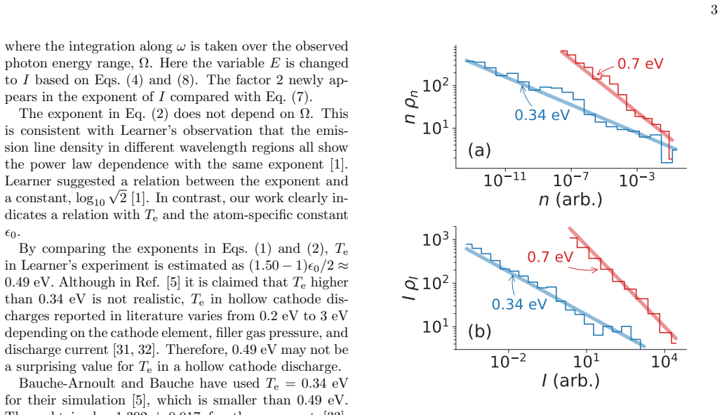
The central discovery is that the long-observed power law in line intensities is not an accident of quantum chaos or fractal structure but a generic statistical consequence of two monotonic functions: an exponentially rising density of states $\rho_E(E) \propto e^{E/\epsilon_0}$ and a Boltzmann population $n_i \propto g_i e^{-E_i/kT_e}$. Mapping the population distribution to a line-intensity distribution, and accounting for the fact that each transition involves two levels (hence two factors of level density), yields $\rho_I(I) \propto I^{-2kT_e/\epsilon_0-1}$. The exponent therefore carries physical meaning: it is a linear measurement of electron temperature divided by the level-density scale. The paper further establishes that the exponent is independent of the observed wavelength window and of instrumental sensitivity, and it confirms the prediction by ab initio collisional-radiative simulation of neutral iron and by power-law fits to thorium hollow-cathode spectra.
Load-bearing premise
The result stands on the assumption that the excited-state population is Boltzmann-distributed at the electron temperature; when collisions are too infrequent to enforce this, the inferred temperature is biased low.
Editorial extensions
If this is right
- The exponent of the line-intensity histogram gives electron temperature directly, without identifying individual lines or knowing oscillator strengths and collision cross sections.
- The method needs only the level-density scale $\epsilon_0$ of the dominant emitter, so it works for atoms such as thorium where conventional radiative data are missing.
- The power law and its exponent survive changes in wavelength window and detector sensitivity, so no absolute intensity calibration is required.
- The same reasoning should apply to any fermionic many-body system whose level density rises exponentially and whose population is thermalized, including heavy nuclei.
Reading between the lines
- A natural next test is to apply the exponent-temperature relation to open-shell elements in well-characterized local-thermal-equilibrium plasmas; agreement would make the diagnostic quantitative, while disagreement would localize the breakdown to the constant-transition-rate approximation.
- The supplementary effective-temperature model suggests that the density-dependent bias at lower electron densities could, in principle, be inverted to estimate electron density as well as temperature.
- The scale-free character implies the same exponent should appear across widely separated spectral regions of one plasma; checking this with a broadband spectrometer would test the ergodic claim more stringently than the wavelength-limited thorium data do.
Signed reviews
Editorial analysis
A structured set of objections, weighed in public.
Referee Report
Summary. The manuscript offers an analytic explanation of Learner's power-law distribution of line intensities in complex many-electron atoms. By combining an exponentially increasing level density with a Boltzmann population distribution, the authors derive ρ_I(I) ∝ I^{-2 k T_e / ϵ_0 - 1}, where T_e is the electron temperature and ϵ_0 the level-density growth scale. They test the result with FAC collisional-radiative simulations for neutral iron and apply it to thorium hollow-cathode spectra to estimate T_e. The derivation is clean, and the FAC simulation reproduces the intermediate population and intensity histograms without imposing the two assumptions. The principal weakness is that whenever the excited-state population is not in full LTE, the exponent is controlled by an effective population temperature T_eff rather than T_e; the paper's own supplementary model quantifies this bias, so the thorium estimates are not unambiguously electron temperatures. The final sentence concedes that LTE validity needs further investigation, but the abstract and conclusion state the diagnostic claim more strongly.
Significance. If the result holds, it provides the first simple analytic explanation of a 40-year-old empirical law and yields a falsifiable, calibration-free diagnostic that avoids line assignment and detailed atomic data. The FAC simulations are a genuine strength: they do not assume the exponential level density or LTE and still reproduce the key features, providing ab initio support for the shape of the relation. The derivation is transparent and the connection to Porter-Thomas line-strength statistics is handled correctly in the Supplementary Material. However, the central diagnostic message—that the measured exponent gives the electron temperature—is not yet validated, because the supplementary analysis shows a density-dependent bias toward T_eff < T_e and the thorium data lack independent checks of T_e and n_e. The paper therefore needs a substantial qualification of its central claim before it can be accepted as a plasma diagnostic.
major comments (3)
- [Supplementary, 'Bias in the Te estimation' (Eq. S25, Fig. S1); main text thorium application] The exponent in Eq. (2) is controlled by the effective population temperature T_eff, not by T_e, whenever the population is not in full LTE. The paper's own collisional-radiative model shows, for Fe at T_e = 0.34 eV and n_e = 10^17 m^-3, that T_eff ≈ 0.7 T_e, and the LTE criterion Eq. (S27) is not far above typical hollow-cathode and divertor conditions. The thorium spectra are from a hollow-cathode plasma with no measured n_e and no independent LTE verification, so the reported values 0.24 ± 0.01 eV and 0.21 ± 0.01 eV are estimates of T_eff, not demonstrated electron temperatures. Because the abstract and conclusion state that the exponent yields the electron temperature, the diagnostic claim is stronger than the evidence supports. Please either reframe the claims in terms of T_eff or add a validation case with independently known T_e and n_e.
- [Main text, Fig. 2 and preceding paragraph] The comparison lines in Fig. 2 are evaluated at T_eff = 0.32 eV and 0.61 eV, the effective temperatures obtained by least-squares fitting of the same simulated population shown in Fig. 1(b), rather than at the actual simulation temperatures T_e = 0.34 eV and 0.70 eV. This validates the internal consistency of Eqs. (7) and (2)—the mapping from an exponential population to an intensity power law—but it does not independently confirm the identification of the measured exponent with 2 k T_e / ϵ_0. Using the true T_e values would change the predicted slopes by roughly 6% and 13% for the two cases. Please state this limitation explicitly and, if possible, show in a figure how the FAC histogram compares with the T_e-based prediction.
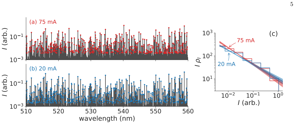
- [Main text, thorium application] The thorium analysis assumes that 'most of the lines are from neutral thorium' even though many lines in the spectra are unidentified and the plasma is a thorium-argon hollow cathode. Because the exponent depends on the emitting species through ϵ_0, an admixture of argon or Th II lines with different ϵ_0 values would bias the fitted slope and hence the inferred temperature. Please quantify the sensitivity to line identification, for example by repeating the fit on subsets of lines known to be Th I or by estimating the contamination fraction needed to change the exponent by the quoted uncertainty.
minor comments (5)
- [Main text, Eq. (6)] The statistical weight g_i is omitted with a one-line statement that it is uniformly distributed over energy; this is an assumption, and the main text should say explicitly that the result holds when g_i is independent of energy, as the Supplementary Material does.
- [Main text, Porter-Thomas paragraph] The sentence that the Porter-Thomas distribution 'decays considerably faster than the power law' is imprecise because the relevant comparison is between the line-strength distribution and s^{-α-1} after marginalization over intensities, as derived in the Supplementary Eq. (S13). Please add a cross-reference to the Supplementary derivation.
- [Fig. 2 caption] The phrase 'the vertical values are multiplied by I' is confusing; the plotted quantities are I ρ_I(I) and n ρ_n(n), not the vertical axis values themselves. Please clarify the caption.
- [Thorium application, maximum-likelihood fits] The quoted uncertainties 1.71 ± 0.03 and 1.64 ± 0.03 are not identified as one standard deviation, while the figure caption mentions 2-σ bands. Please specify the confidence level for the reported exponents.
- [Supplementary, Eq. (S13)] The power law is derived under the condition I ≫ I_min; since observed histograms cover a finite dynamic range, please state the intensity range over which the power law is expected to hold and confirm that the thorium and iron histograms fall within that range.
Circularity Check
No significant circularity: the intensity power law is derived from independent level-density data and the LTE population assumption, and the thorium temperatures are inferred from external ϵ0 values, not fitted to the target.
full rationale
The central derivation (Eqs. (3), (4), (7), (2)) takes two stated inputs — exponential level density ρ_E(E)∝exp(E/ϵ0) and Boltzmann population n_i∝g_i exp(-E_i/kTe) — and derives the line-intensity power law ρ_I(I)∝I^{-2kTe/ϵ0-1} by a change of variables and an integration over photon energies. Neither input is defined in terms of the intensity histogram; ϵ0 for iron is fitted to the simulated level density (Fig. 1(a)) and for thorium is taken from external work by Dzuba and Flambaum [9]. The measured thorium exponents are then used to estimate Te via Eq. (2), which is a diagnostic application, not a circular validation. The FAC simulations are genuine ab initio checks: the paper explicitly states that 'in the FAC computations we do not explicitly adopt either of our two assumptions,' and the population and intensity distributions are compared with, not fitted to, the theoretical lines. The effective temperatures 0.32 eV and 0.61 eV are least-squares fits to the energy dependence of the simulated population, and using the same values to draw Eq. (7) and Eq. (2) is a self-consistency transformation rather than a fit to the plotted intensity histogram; any imperfection would show as disagreement. No load-bearing self-citation occurs: the key references (Learner 1982, Dzuba & Flambaum 2010, Porter & Thomas 1956) are external, and the present authors do not cite themselves for the central premise. The paper's own caveat that 'the validity of the local thermal equilibrium assumption should be investigated further' is a correctness/robustness limitation about LTE in real plasmas, not a circularity: it does not make Eq. (2) equivalent to its inputs. The derivation is self-contained relative to the targets it predicts.
Assumptions & free parameters
free parameters (2)
- epsilon_0 (level-density growth energy) =
1.97 +/- 0.04 eV for neutral iron (MLE of FAC levels); 0.68 eV for neutral thorium from Ref. [9]
- T_eff (effective population temperature) =
0.32 eV and 0.61 eV for the FAC iron cases
assumptions (3)
- domain assumption Excited-level density of complex atoms grows exponentially with energy, rho_E(E) proportional to exp(E/epsilon_0) below ionization (Eq. 3).
- domain assumption Excited-state populations follow a Boltzmann distribution at electron temperature T_e (Eq. 4).
- domain assumption Line strengths are independent and identically distributed with a distribution that decays faster than a power law; approximated by a constant S0 (Eq. 8 and supplementary).
Cite this review
Pith. "Pith review of A Simple Explanation for the Observed Power Law Distribution of Line Intensity in Complex Many-Electron Atoms." pith.science (2026). https://pith.science/paper/QGVPM6LL
@misc{pith2026190810464,
  author       = {Pith},
  title        = {Pith review of: A Simple Explanation for the Observed Power Law Distribution of Line Intensity in Complex Many-Electron Atoms},
  year         = {2026},
  howpublished = {\url{https://pith.science/paper/QGVPM6LL}},
  note         = {Machine review of arXiv:1908.10464}
}
read the original abstract
It has long been observed that the number of weak lines from many-electron atoms follows a power law distribution of intensity. While computer simulations have reproduced this dependence, its origin has not yet been clarified. Here we report that the combination of two statistical models -- an exponential increase in the level density of many-electron atoms and local thermal equilibrium of the excited state population -- produces a surprisingly simple analytical explanation for this power law dependence. We find that the exponent of the power law is proportional to the electron temperature. This dependence may provide a useful diagnostic tool to extract the temperature of plasmas of complex atoms without the need to assign lines.
Figures

Reference graph
Works this paper leans on
-
[1]
R. C. M. Learner, Journal of Physics B: Atomic and Molecular Physics 15, L891 (1982)
work page 1982
-
[2]
Note that although he used a different base, 2 for the intensity and 10 for the line number, we usee as the base and present the converted value by b log 10/ log 2 − 1 for later convenience, where b is the original value, -0.15
-
[3]
Scheeline, Analytical Chemistry 58, 3103 (1986)
A. Scheeline, Analytical Chemistry 58, 3103 (1986)
work page 1986
-
[4]
Scheeline, Analytical Chemistry 58, 802 (1986)
A. Scheeline, Analytical Chemistry 58, 802 (1986)
work page 1986
-
[5]
C. Bauche-Arnoult and J. Bauche, Journal of Quantita- tive Spectroscopy and Radiative Transfer 58, 441 (1997)
work page 1997
-
[6]
Pain, High Energy Density Physics 9, 392 (2013)
J.-C. Pain, High Energy Density Physics 9, 392 (2013)
work page 2013
- [7]
-
[8]
V. V. Flambaum, A. A. Gribakina, and G. F. Gribakin, Physical Review A 58, 230 (1998)
work page 1998
Show all 43 references
-
[9]
V. A. Dzuba and V. V. Flambaum, Physical Review Let- ters 104, 213002 (2010), arXiv:1003.4576
2010 arXiv
-
[10]
H. R. Griem, Fast Electrical and Optical Measurements (Springer Netherlands, Dordrecht, 1986) pp. 885–910
1986
-
[11]
Fujimoto, Plasma Polarization Spectroscopy (Springer Berlin Heidelberg, Berlin, Heidelberg) pp
T. Fujimoto, Plasma Polarization Spectroscopy (Springer Berlin Heidelberg, Berlin, Heidelberg) pp. 29–49
-
[12]
Sawada, K
K. Sawada, K. Eriguchi, and T. Fujimoto, Journal of Applied Physics 73, 8122 (1993)
1993
-
[13]
Goto, Journal of Quantitative Spectroscopy and Ra- diative Transfer 76, 331 (2003)
M. Goto, Journal of Quantitative Spectroscopy and Ra- diative Transfer 76, 331 (2003)
2003
-
[14]
B¨ owering, M
N. B¨ owering, M. Martins, W. N. Partlo, and I. V. Fomenkov, Journal of Applied Physics 95, 16 (2004)
2004
-
[15]
Masnavi, M
M. Masnavi, M. Nakajima, E. Hotta, K. Horioka, G. Ni- imi, and A. Sasaki, Journal of Applied Physics 101, 033306 (2007)
2007
-
[16]
Suzuki, F
C. Suzuki, F. Koike, I. Murakami, N. Tamura, and 5 10 3 10 1 I (arb.) (a) 75 mA 510 520 530 540 550 560 wavelength (nm) 10 3 10 1 I (arb.) (b) 20 mA 10 2 10 1 100 I (arb.) 101 102 103 I I 75 mA 20 mA (c) FIG. 3. Emission spectra observed from thorium-argon hollow cathode plasm...
2012
-
[17]
P¨ utterich, R
T. P¨ utterich, R. Neu, R. Dux, A. D. Whiteford, and M. G. O’Mullane, Plasma Physics and Controlled Fusion 50, 085016 (2008)
2008
-
[18]
Murakami, H
I. Murakami, H. Sakaue, C. Suzuki, D. Kato, M. Goto, N. Tamura, S. Sudo, and S. Morita, Nuclear Fusion 55, 093016 (2015)
2015
-
[19]
E. Pian, P. D’Avanzo, S. Benetti, M. Branchesi, E. Bro- cato, S. Campana, E. Cappellaro, S. Covino, V. D’Elia, J. P. U. Fynbo, F. Getman, G. Ghirlanda, G. Ghis- ellini, A. Grado, G. Greco, J. Hjorth, C. Kouveliotou, A. Levan, L. Limatola, D. Malesani, P. A. Mazzali, A. Melandr...
2017
-
[20]
Tanaka, D
M. Tanaka, D. Kato, G. Gaigalas, P. Rynkun, L. Radˇ zit, S. Wanajo, Y. Sekiguchi, N. Nakamura, H. Tanuma, I. Murakami, and H. A. Sakaue, The Astrophysical Jour- nal 852, 109 (2018), arXiv:1708.09101
2018 arXiv
-
[21]
NIST Atomic Spectra Database (version 5.6.1),
A. Kramida, Y. Ralchenko, J. Reader, and N. A. T. (2018), “NIST Atomic Spectra Database (version 5.6.1),” (https://physics.nist.gov/asd), [Accessed: 8-Feb-2019]
2018
-
[22]
M. F. Gu, Canadian Journal of Physics 86, 675 (2008)
2008
-
[23]
Ter Haar, Physical Review 76, 1525 (1949)
D. Ter Haar, Physical Review 76, 1525 (1949)
1949
-
[24]
Von Egidy, A
T. Von Egidy, A. N. Behkami, and H. H. Schmidt, Nu- clear Physics , Tech. Rep. (1986)
1986
-
[25]
M. V. Simkin and V. P. Roychowdhury, Physics Reports 502, 1 (2011)
2011
-
[26]
C. E. Porter and R. G. Thomas, Physical Review 104, 483 (1956)
1956
-
[27]
S. M. Grimes, Physical Review C 28, 471 (1983)
1983
-
[28]
S. E. Bisson, E. F. Worden, J. G. Conway, B. Comaskey, J. A. D. Stockdale, and F. Nehring, Journal of the Op- tical Society of America B 8, 1545 (1991)
1991
-
[29]
V. V. Flambaum, A. A. Gribakina, G. F. Gribakin, and M. G. Kozlov, Phys. Rev. A 50, 267 (1994)
1994
-
[30]
(2), as well as the validity condition of the local- thermal-equilibrium assumption, which includes Refs
See Supplementary Material for more detailed derivation of Eq. (2), as well as the validity condition of the local- thermal-equilibrium assumption, which includes Refs. [8, 26–28, 37–43]
-
[31]
D. M. Mehs and T. M. Niemczyk, Applied Spectroscopy 35, 66 (1981)
1981
-
[32]
L. Meng, R. Raju, R. Flauta, H. Shin, D. N. Ruzic, and D. B. Hayden, Journal of Vacuum Science & Technology A: Vacuum, Surfaces, and Films 28, 112 (2010)
2010
-
[33]
This value is also converted from the original value b = −0.118 ± 0.005
-
[34]
Palmer and R
B. Palmer and R. J. Engleman, Atlas of the thorium spectrum, Tech. Rep. (Los Alamos National Laboratory (LANL), Los Alamos, NM, 1980)
1980
-
[35]
Kerber, G
F. Kerber, G. Nave, and C. J. Sansonetti, The Astro- physical Journal Supplement Series 178, 374 (2008)
2008
-
[36]
Kitt Peak National Observatory Data Archives,
“Kitt Peak National Observatory Data Archives,” ftp: //nispdata.nso.edu, [Accessed: 23-Nov-2019]
2019
-
[37]
Mewe, Astronomy and Astrophysics 20, 215 (1972)
R. Mewe, Astronomy and Astrophysics 20, 215 (1972)
1972
-
[38]
H. R. Griem, Physical Review 131, 1170 (1963)
1963
-
[39]
McWhirter, in Plasma DiagnosticTechniques, edited by R
R. McWhirter, in Plasma DiagnosticTechniques, edited by R. Huddlestone and S. Leonard (Academic Press, New York, 1965) pp. 201–264
1965
-
[40]
Suzuki, T
C. Suzuki, T. Higashiguchi, A. Sasanuma, G. Arai, Y. Fujii, Y. Kondo, T.-H. Dinh, F. Koike, I. Murakami, and G. O’Sullivan, Nuclear Instruments and Methods in Physics Research Section B: Beam Interactions with Ma- terials and Atoms 408, 253 (2017)
2017
-
[41]
O’sullivan, B
G. O’sullivan, B. Li, R. D ’arcy, P. Dunne, P. Hay- 6 den, D. Kilbane, T. Mccormack, H. Ohashi, F. O ’reilly, P. Sheridan, E. Sokell, C. Suzuki, and T. Higashiguchi, Journal of Physics B: Atomic, Molecular and Optical Physics J. Phys. B: At. Mol. Opt. Phys 48, 144025 (2015)
2015
-
[42]
Kawashima, K
H. Kawashima, K. Shimizu, T. Takizuka, K. Tobita, S. Nishio, S. Sakurai, and H. Takenaga, Nuclear Fusion 49, 065007 (2009)
2009
-
[43]
effective charge
A. Kukushkin, H. Pacher, V. Kotov, G. Pacher, and D. Reiter, Fusion Engineering and Design 86, 2865 (2011). A Simple Explanation for the Observed Power Law Distribution of Line Intensity in Complex Many-Electron Atoms DET AILED DERIV A TION OF THE INTENSITY DISTRIBUTION In the...
2011
Reviewed August 14, 2026 · model on record in the stance chip above.
Discussion (0). Continue with ORCID to comment.