REVIEW 5 major objections 4 minor 38 references
Growth Dynamics of Value and Cost Trade-off in Temporal Networks
T0 review · 5 major / 4 minor · reviewed 2026-08-14 · deepseek-v4-flash
Pith's one-line read A preferential-attachment network that must pay per link either fails immediately, grows without bound, or enters a trade-off; the trade-off split sits at $\alpha=3m$.
desk verdict The paper asks a good question but its value-growth equation violates the stated link budget, so the α=3m boundary and the ever-growing scenario don't survive correction. read the letter →
The pith
A machine-rendered reading of the paper's core claim, the machinery that carries it, and where it could break.
The reading
What carries the argument
The machinery is a two-curve race. The value of a node's accumulated links is $k_v(t)=2mt+c\sqrt{t}$, and the cumulative cost of its attachments is $k_c(t)=(\alpha+m)t$, with $m$ links added per time step, $c$ fixed by the initial degree, and $\alpha$ a free linear cost slope. Growth is the condition $k_v-k_c>0$; stopping happens at the characteristic time $t_{\mathrm{char}}=(c/(\alpha-m))^2$ where the curves meet. The value curve itself changes behaviour at the cross-over time $t_*=c^2/(4m^2)$, going from $\sqrt{t}$-like to linear. Setting $t_{\mathrm{char}}=t_*$ gives $\alpha=3m$ (with the negative root $\alpha=-m$ discarded), and that equality partitions the phase space into the paper's three scenarios.
What would settle it
Track a real growing temporal network in which attachment costs can be observed, fit the cumulative cost of links over time, and check whether it is linear with slope $\alpha+m$. If the best-fit scaling is not linear, the phase diagram collapses. A sharper check: estimate $\alpha$ and $m$ from data and test whether networks with $m<\alpha<3m$ first accelerate and then stop at $t_{\mathrm{char}}=c^2/(\alpha-m)^2$, while networks with $\alpha>3m$ stop before the value acceleration.
Extended reading notes
Core claim
On the paper's own terms, preferential attachment alone does not explain why real networks stop growing, so the paper adds a per-attachment cost. It takes the value of a node's accumulated links to be $k_v(t)=2mt+c\sqrt{t}$ and the cumulative cost of attachments to be $k_c(t)=(\alpha+m)t$, where $m$ is the number of new links per time step, $c$ encodes the initial degree, and $\alpha$ is a free cost parameter. Growth continues while $k_v-k_c>0$ and stops at the characteristic time $t_{\mathrm{char}}=(c/(\alpha-m))^2$. Comparing $t_{\mathrm{char}}$ with the value's cross-over time $t_*=c^2/(4m^2)$—the moment the value curve shifts from $\sqrt{t}$-like to linear—gives the equation $\alpha=3m$ (and the ineligible root $\alpha=-m$). The paper therefore claims three fates: immediate failure when $\alpha\gg m$; unbounded growth when $\alpha$ approaches $m$ from below; and a trade-off in between, split into networks that stop before the value acceleration ($\alpha>3m$) and networks that accelerate and then stop ($m<\alpha<3m$).
Load-bearing premise
The classification rests on the assumed exact linear cost law $k_c(t)=(\alpha+m)t$; the paper neither derives this law from micro-behaviour nor measures it, so if real attachment costs grow superlinearly, sublinearly, or depend on degree, the predicted regimes and the $\alpha=3m$ boundary no longer follow.
Editorial extensions
If this is right
- Any preferential-attachment network with a positive linear cost slope $\alpha>m$ will eventually stop growing, because the characteristic time exists and growth ends when the cost curve crosses the value curve.
- The dividing line between never stopping and eventually stopping is $\alpha=m$; the safest growth strategy is to keep the cost rate at or below the link creation rate, and the paper identifies $0\le \alpha/m \le 3$ as the window that avoids outright early failure.
- Within the trade-off region, networks with $\alpha>3m$ die before the value curve accelerates, while those with $m<\alpha<3m$ enjoy an accelerating phase and then stall, predicting an observable boom-then-stop pattern.
- Because higher $m$ shortens both the cross-over time and the characteristic time, faster link creation accelerates the network's evolution toward its eventual stop rather than postponing it.
- In economic applications, the model gives a quantitative criterion for when a platform stops being worth joining: once the cost slope $\alpha$ exceeds $m$, the marginal value of new links falls below their cumulative cost at a predictable time.
Reading between the lines
- Beyond the paper, if $\alpha$ is allowed to vary over time, the $\alpha=3m$ boundary becomes a moving threshold and the network could switch repeatedly between accelerating and stalling—a cyclic growth regime the paper does not consider.
- Beyond the paper, separating the lumped cost $\alpha$ into an internal structural part and an external competition part would yield distinct stopping times and could be fit independently to data from organizations versus markets.
- Beyond the paper, the safe window $0\le \alpha/m\le 3$ suggests a practical monitoring rule: track the ratio of per-attachment cost to per-step recruitment; approaching $\alpha=m$ warns that the no-growth boundary is near.
- Beyond the paper, in financial networks this predicts that aggregate growth can accelerate and then reverse with constant individual leverage, because the stall is driven by cumulative attachment cost rather than by balance-sheet leverage.
Signed reviews
Editorial analysis
A structured set of objections, weighed in public.
Referee Report
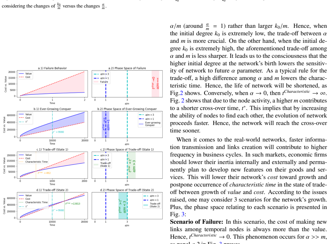
Summary. The paper proposes a growth model for temporal networks in which preferential attachment is combined with a cost of link creation. It defines per-node value as kv(t) = 2mt + c√t (Eq. 3), posits a linear cost kc(t) = (α+m)t (Eq. 8), and derives a characteristic time t_characteristic = (c/(α−m))^2 (Eq. 9) at which cost overtakes value. Equalizing this with the value cross-over time t* (Eq. 6) yields Eq. (10), giving α = 3m as the boundary between two trade-off states. The paper then classifies network fates into failure (α >> m), two trade-off states (α > 3m and α < 3m), and ever-growing behavior (α/m → 1), and claims that a trade-off between value and cost emerges under these conditions.
Significance. If the model were correct, it would provide a simple analytical explanation for why real-world networks may stop growing, with explicit thresholds and a falsifiable three-scenario classification. The paper deserves credit for formulating a clear value/cost trade-off question and for deriving closed-form expressions for characteristic times. However, the central derivation is inconsistent with the network process it claims to model, and the scenario classification is internally contradictory. No simulations, empirical data, or error estimates are provided. Because the main results (Eqs. 6, 9, 10) follow from an incorrect mean-field equation and an unvalidated cost ansatz, the significance of the claimed findings is not currently established.
major comments (5)
- [Section 4, Eq. (2)] The mean-field rate equation does not correspond to the process stated in the same section. The process selects m nodes uniformly among N at each time step, each creating one link, so a given node is a source with probability m/N, not m. Summing Eq. (2) over all nodes gives Σ dk_i/dt ≈ m(N+1), whereas the network's total degree grows at rate 2m per step. Consequently, the solution Eq. (3), kv = 2mt + c√t, overstates per-node degree by a factor of order N and violates the link budget. With the correct source rate m/N, the value term becomes (2m/N)t + c√t, the characteristic time becomes c^2/(α + m − 2m/N)^2, and for N > 2 perpetual growth would require α < 0, contradicting the paper's 'ever-growing' scenario near α ≈ m. Every subsequent quantity (Eqs. 6, 9, 10) inherits this error.
- [Section 4, Eq. (8)] The cost function kc(t) = (α+m)t is introduced without derivation or justification. α is a free parameter with no stated microscopic or empirical origin, and the phrase 'α is the phase space' does not define it. The entire scenario classification, including the α = 3m boundary (Eq. 10), is a consequence of assuming an exactly linear cost in time. The paper never tests this assumption against a cost-generating mechanism (e.g., competition cost or structural cost) nor against data, so the claimed trade-off is conditional on an unvalidated ansatz.
- [Section 5, Eqs. (10)-(12) and 'Scenario of Ever-growing Conquer'] The classification is internally inconsistent. From Eq. (9), t_characteristic is finite whenever α ≠ m (assuming c ≠ 0). For α > m, growth stops at a finite time; for α < m, the intersection of kv and kc is the point where value overtakes cost, not where growth stops. Thus perpetual growth occurs for α ≤ m (for c > 0 at large t), not merely 'α/m → 1'. Moreover, Eq. (12) places all α < 3m in the second trade-off state, which includes α ≈ m; this contradicts the paper's claim that α/m → 1 gives the ever-growing scenario. The correct boundary between perpetual growth and eventual stagnation is α = m, not α = 3m.
- [Section 4, Eq. (4)] The constant c = (k0 − 2m t0)/√t0 contains an undefined initial time t0 and is singular at t0 = 0. The paper never specifies the domain of validity of Eq. (3), nor the sign of c. If c < 0, then kv(t) is negative for small t, which is unphysical for a degree. These issues affect the interpretation of t* and t_characteristic and need to be resolved before the scenario analysis can be accepted.
- [General (no section)] The manuscript provides no numerical simulation or empirical validation of the predicted scenarios. Because the analytical derivation is the sole basis of the claims and contains the inconsistencies detailed above, the predicted growth fates are not verified. A simulation of the stated network process, or a fit to a real temporal network dataset, is needed to determine whether any of the described regimes actually occur.
minor comments (4)
- [Eq. (8)] The first line of Eq. (8) writes kν(t) using a Greek nu, while the text elsewhere uses kv; please unify the notation.
- [Section 4] The phrase 'α is the phase space' is unclear and unconventional; replace it with a clear description of α as a cost-growth coefficient with defined units.
- [Abstract and throughout] The manuscript contains numerous typographical and grammatical errors, including 'statue quo' (Section 3), 'Agancy Theory' (Section 3), 'di erent' (Abstract), and 'trade-o ' throughout; it needs careful proofreading.
- [Fig. 3] The text refers to panels a.2, b.1, b.2, c, and d of Fig. 3, but the panel labels are not described in the text; please add a legend or caption explaining each panel.
Circularity Check
No significant circularity: the scenario boundaries follow algebraically from the paper's stated differential equations.
full rationale
The paper's derivation chain is self-contained conditional on its stated assumptions. Equation (3) is presented as the analytical solution of Equation (2), the stated mean-field rate for node activity, and Equation (9) is obtained by solving the equality kv=kc. The trade-off boundaries in Equations (10)-(12) are direct algebraic consequences of comparing t_characteristic with t*; the value of α=3m is not inserted as an input and no fitted parameter is relabeled as a prediction. The cost function kc=(α+m)t in Equation (8) is indeed an ansatz with no microscopic or empirical derivation, and the value equation may be inconsistent with the network's link budget (a correctness concern), but neither issue makes the derivation circular: the paper does not fit α to the scenario outcomes and then rediscover those outcomes. The citation to [4], a coauthored prior paper, is used as a source for the activity model, but Equations (2)-(3) are re-derived in the text, so this self-citation is not load-bearing in a circularity sense. No step in the paper reduces by construction to its own input.
Assumptions & free parameters
free parameters (5)
- α (cost growth coefficient)
- c (initial condition constant) =
c=(k0-2m t0)/√t0, t0 undefined
- m (links created per time step)
- k0 (initial degree)
- t0 (initial time)
assumptions (5)
- domain assumption Mean-field preferential attachment rate equation dki/dt = m + m ki/Σj≠i kj (Eq. 2) governs node value growth.
- standard math Total degree sum can be approximated as 2mt, with initial links neglected.
- ad hoc to paper Cost of attachments grows exactly linearly with time, kc=(α+m)t.
- domain assumption Network fate is fully determined by the sign of kv-kc.
- domain assumption Initial links m0 can be neglected in the solution.
invented entities (1)
-
Cost variable kc(t)
Cite this review
Pith. "Pith review of Growth Dynamics of Value and Cost Trade-off in Temporal Networks." pith.science (2026). https://pith.science/paper/TMFHL7QF
@misc{pith2026190811433,
  author       = {Pith},
  title        = {Pith review of: Growth Dynamics of Value and Cost Trade-off in Temporal Networks},
  year         = {2026},
  howpublished = {\url{https://pith.science/paper/TMFHL7QF}},
  note         = {Machine review of arXiv:1908.11433}
}
read the original abstract
The question is: What does happen to the real-world networks which cause them not to grow permanently? The idea here is that real-world networks have to pay the cost of growth. We investigate the growth and trade-off between value and cost in the networks with cost and preferential attachment together. Since the preferential attachment in the BA model does not consider any stop against the infinite growth of networks, we introduce a modified version of preferential attachment of the BA model. This idea makes sense because the growth of real networks may be finite. In the present study, by combining preferential attachment in the science of temporal networks (interval graphs), and, the first-order differential equations of value and cost of making links, the future equilibrium of an evolving network is illustrated. During the process of achieving a winning position, the variables against growth such as the competition cost, besides the internally structural cost may emerge. In the end, by applying this modified model, we found the circumstances in which a trade-off between value and cost emerges.
Figures


Reference graph
Works this paper leans on
-
[4]
Memory effects on link formation in temporal networks: A fractional calculus approach
F. Rabbani, T. Khraisha, F. Abbasi, G. Jafari, Link formation in aged temporal networks. URL https://arxiv.org/abs/1908.01999
work page Pith review arXiv 1908
-
[1]
A.-L. Barab ´asi, R. Albert, Emergence of scaling in random networks, Sci- ence 286 (5439) (1999) 509–512. doi:10.1126/science.286.5439. 509
-
[2]
A.-L. Barab ´asi, R. Albert, H. Jeong, Mean-field theory for scale-free random networks, Physica A: Statistical Mechanics and its Applications 272 (1-2) (1999) 173–187. doi:10.1016/s0378-4371(99)00291-5
-
[3]
M. E. J. Newman, Clustering and preferential attachment in growing networks, Physical Review E 64 (2). doi:10.1103/physreve.64. 025102
-
[5]
A. H. Shirazi, A. Namaki, A. A. Roohi, G. R. Jafari, Transparency e ffect in the emergence of monopolies in social networks, Journal of Artificial Societies and Social Simulation 16 (1) (2013) 1.doi:10.18564/jasss. 2054
doi:10.18564/jasss 2013
-
[6]
Y . Tang, J. Kurths, W. Lin, E. Ott, L. Kocarev, Introduction to focus issue: When machine learning meets complex systems: Networks, chaos, and nonlinear dynamics, Chaos: An Interdisciplinary Journal of Nonlinear Science 30 (6) (2020) 063151. doi:10.1063/5.0016505. URL https://doi.org/10.1063%2F5.0016505
-
[7]
D. Bianchi, M. Billio, R. Casarin, M. Guidolin, Modeling systemic risk with markov switching graphical SUR models, Journal of Econometrics 210 (1) (2019) 58–74. doi:10.1016/j.jeconom.2018.11.005
-
[8]
M. Bardoscia, S. Battiston, F. Caccioli, G. Caldarelli, Pathways towards instability in financial networks, Nature Communications 8 (1). doi: 10.1038/ncomms14416
Show all 38 references
-
[9]
Ardalankia, J
J. Ardalankia, J. Askari, S. Sheykhali, E. Haven, G. R. Jafari, Mapping coupled time-series onto complex network (2020). arXiv:2004.13536
2020 arXiv
-
[10]
Namaki, J
A. Namaki, J. Ardalankia, R. Raei, L. Hedayatifar, A. Hosseiny, E. Haven, G. Jafari, Analysis of global banking network
-
[11]
Zhao, G.-J
L. Zhao, G.-J. Wang, M. Wang, W. Bao, W. Li, H. E. Stanley, Stock market as temporal network, Physica A: Statistical Mechanics and its Ap- plications 506 (2018) 1104–1112. doi:10.1016/j.physa.2018.05. 039
2018 doi
-
[12]
Etesami, A
J. Etesami, A. Habibnia, N. Kiyavash, Econometric modeling of systemic risk: going beyond pairwise comparison and allowing for nonlinearity, LSE Research Online Documents on Economics 70769, London School of Economics and Political Science, LSE Library (Mar. 2017). URL https:/...
2017
-
[13]
Billio, R
M. Billio, R. Casarin, M. Iacopini, Bayesian markov switching tensor regression for time-varying networks, SSRN Electronic Journaldoi:10. 2139/ssrn.3192341
-
[14]
Lambiotte, M
R. Lambiotte, M. Rosvall, I. Scholtes, From networks to optimal higher- 5 order models of complex systems, Nature Physics 15 (4) (2019) 313–320. doi:10.1038/s41567-019-0459-y
2019 doi
-
[15]
Holme, J
P. Holme, J. Saram ¨aki, Temporal networks, Physics Reports 519 (3) (2012) 97–125. doi:10.1016/j.physrep.2012.03.001
2012 doi
-
[16]
J. M. Buld ´u, F. Pablo-Mart´ı, J. Aguirre, Taming out-of-equilibrium dy- namics on interconnected networks, Nature Communications 10 (1). doi:10.1038/s41467-019-13291-2
-
[17]
Jurczyk, T
J. Jurczyk, T. Rehberg, A. Eckrot, I. Morgenstern, Measuring critical transitions in financial markets, Scientific Reports 7 (1). doi:10.1038/ s41598-017-11854-1
-
[18]
Grauwin, E
S. Grauwin, E. Bertin, R. Lemoy, P. Jensen, Competition between col- lective and individual dynamics, Proceedings of the National Academy of Sciences 106 (49) (2009) 20622–20626. doi:10.1073/pnas. 0906263106
2009 doi
-
[19]
Haller, S
H. Haller, S. Sarangi, Nash networks with heterogeneous links, Math- ematical Social Sciences 50 (2) (2005) 181–201. doi:10.1016/j. mathsocsci.2005.02.003
2005 doi
-
[20]
P. L. Krapivsky, S. Redner, F. Leyvraz, Connectivity of growing random networks, Physical Review Letters 85 (21) (2000) 4629–4632. doi:10. 1103/physrevlett.85.4629
2000
-
[21]
P. L. Krapivsky, S. Redner, Organization of growing random networks, Physical Review E 63 (6). doi:10.1103/physreve.63.066123
-
[22]
Bianconi, A.-L
G. Bianconi, A.-L. Barab ´asi, Competition and multiscaling in evolving networks, Europhysics Letters (EPL) 54 (4) (2001) 436–442. doi:10. 1209/epl/i2001-00260-6
2001
-
[23]
Iranzo, J
J. Iranzo, J. M. Buld ´u, J. Aguirre, Competition among networks high- lights the power of the weak, Nature Communications 7 (1). doi: 10.1038/ncomms13273
-
[24]
Aguirre, D
J. Aguirre, D. Papo, J. M. Buld ´u, Successful strategies for compet- ing networks, Nature Physics 9 (4) (2013) 230–234. doi:10.1038/ nphys2556
2013
-
[25]
J. Liu, J. Li, Y . Chen, X. Chen, Z. Zhou, Z. Yang, C.-J. Zhang, Model- ing complex networks with accelerating growth and aging effect, Physics Letters Adoi:10.1016/j.physleta.2019.02.004
2019 doi
-
[26]
S. N. Dorogovtsev, J. F. F. Mendes, Evolution of networks, Ad- vances in Physics 51 (4) (2002) 1079–1187. doi:10.1080/ 00018730110112519
2002
-
[27]
Ikeda, Topology of growing networks accelerated by intermediary pro- cess, Physica A: Statistical Mechanics and its Applications 484 (2017) 378–393
N. Ikeda, Topology of growing networks accelerated by intermediary pro- cess, Physica A: Statistical Mechanics and its Applications 484 (2017) 378–393. doi:10.1016/j.physa.2017.04.123
2017 doi
-
[28]
Safdari, M
H. Safdari, M. Z. Kamali, A. Shirazi, M. Khalighi, G. Jafari, M. Ausloos, Fractional dynamics of network growth constrained by aging node inter- actions, PLOS ONE 11 (5) (2016) e0154983. doi:10.1371/journal. pone.0154983
2016 doi
-
[29]
Vardanyan, D
E. Vardanyan, D. B. Saakian, The analytical dynamics of the finite popu- lation evolution games, Physica A: Statistical Mechanics and its Applica- tions (2020) 124233doi:10.1016/j.physa.2020.124233
2020
-
[30]
Khalighi, J
M. Khalighi, J. Ardalankia, A. K. Rizi, H. Ebadi, G. Jafari, Opti- mized memory reveals the survival strategy for a multi-agent competition (2019). arXiv:1908.03076
2019 arXiv
-
[31]
Cohen, K
R. Cohen, K. Erez, D. ben Avraham, S. Havlin, Resilience of the internet to random breakdowns, Physical Review Letters 85 (21) (2000) 4626–
2000
-
[32]
Zhang, B
T. Zhang, B. Fang, X. Liang, A novel measure to identify influen- tial nodes in complex networks based on network global e fficiency, Modern Physics Letters B 29 (28) (2015) 1550168. doi:10.1142/ s0217984915501687
2015
-
[33]
Joshi, A
S. Joshi, A. S. Mahmud, S. Sarangi, Network formation with multigraphs and strategic complementarities, Journal of Economic Theory 188 (2020) 105033. doi:10.1016/j.jet.2020.105033
2020
-
[34]
Fronczak, J
A. Fronczak, J. A. Hołyst, M. Jedynak, J. Sienkiewicz, Higher order clustering coefficients in barab ´asi–albert networks, Physica A: Statisti- cal Mechanics and its Applications 316 (1-4) (2002) 688–694. doi: 10.1016/s0378-4371(02)01336-5
2002 doi
-
[35]
Chmiel, J
A. Chmiel, J. A. Hołyst, Transition due to preferential cluster growth of collective emotions in online communities, Physical Review E 87 (2). doi:10.1103/physreve.87.022808
-
[36]
M. D. Chari, P. David, A. Duru, Y . Zhao, Bowman’s risk-return paradox: An agency theory perspective, Journal of Business Research 95 (2019) 357–375. doi:10.1016/j.jbusres.2018.08.010
2019 doi
-
[37]
Naeem, M
K. Naeem, M. C. Li, Corporate investment e fficiency: The role of finan- cial development in firms with financing constraints and agency issues in OECD non-financial firms, International Review of Financial Analysis 62 (2019) 53–68. doi:10.1016/j.irfa.2019.01.003. 6
2019 doi
-
[4628]
doi:10.1103/physrevlett.85.4626
Reviewed August 14, 2026 · model on record in the stance chip above.
Discussion (0). Continue with ORCID to comment.