REVIEW 2 major objections 5 minor 48 references
Edge tracking in spatially developing boundary layer flows
T0 review · 2 major / 5 minor · reviewed 2026-08-14 · deepseek-v4-flash
Pith's one-line read A moving box lets edge trajectories in a Blasius boundary layer reveal streak switching, Tollmien–Schlichting waves, and the edge as a divider of two transition routes.
desk verdict A genuinely useful moving-box technique and first streak switching in the Blasius edge, but the validation of the technique is too thin and the coexistence claim is slightly ahead of the data. read the letter →
The pith
A machine-rendered reading of the paper's core claim, the machinery that carries it, and where it could break.
The reading
What carries the argument
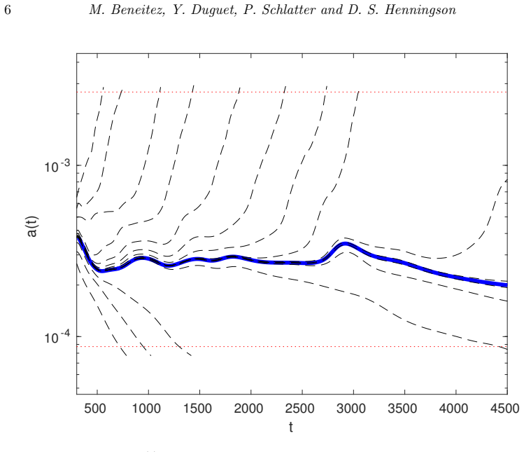
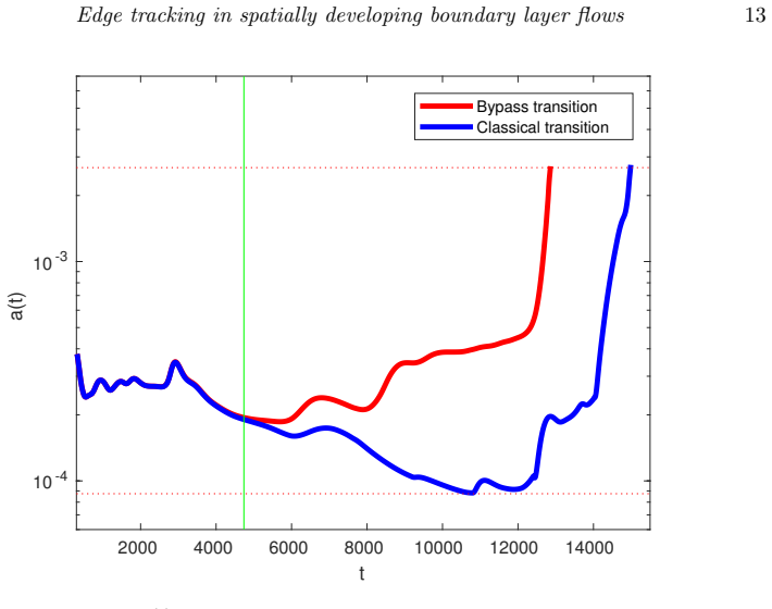
The machinery is the moving box technique combined with bisection on a specially chosen observable. The box translates streamwise at piecewise-constant speed $c_{\mathrm{box}}$ (here alternating between 0 and $0.8U_\infty$), implemented by Galilean transformations of the velocity and by updating the Blasius base flow used in the fringe (damping) region at the outflow, so the localized structure remains inside a domain of length $L_x=6000$ for times that would otherwise need a box twice as long; this extends the tracking horizon roughly threefold compared with earlier Blasius edge computations. The scalar observable used in the bisection is the volume-averaged root-mean-square of the streamwise vorticity, which vanishes for the laminar profile and is exactly zero for spanwise-invariant TS waves in their linear stage, so the bisection continues to bracket the edge even after the base-flow instability has set in. These two elements produce a finite-time edge trajectory that stays spatially localized, scales with the local displacement thickness $\delta^*(x_G(t))$, and lives long enough for streak switching and the later coexistence of TS waves with the streak core.
What would settle it
Perform the same edge-bracketing bisection in a fixed domain of size $(L_x,L_y,L_z)=(12000,60,100)$ with the same resolution and compare, up to $t\approx 4700$, the observable $a(t)$, the streak-switch times, the structure position $x_G(t)$, and the TS wave crest trajectories against the moving-box run; if the trajectories differ by more than the bisection uncertainty ($\delta\lambda/\lambda^*\sim 10^{-4}$) in any of these diagnostics, the equivalence between moving and fixed boxes fails.
Extended reading notes
Core claim
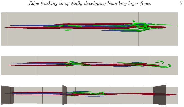
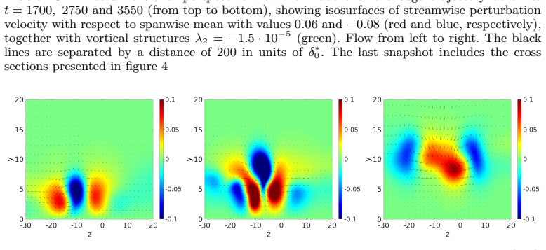
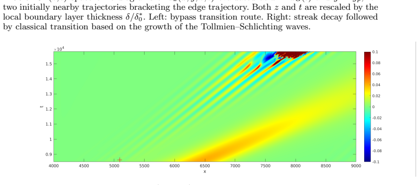
The central discovery is that both classical and bypass transition mechanisms can be reached from a single finite-time trajectory on the edge manifold, selected by bisection in the amplitude of an initial pair of counter-rotating vortices. At moderate times the trajectory is a localized self-sustained streaky structure that regenerates and switches the sign of its central streak, with no discrete symmetry imposed. At long times, varying the bisection parameter by a relative amount of order $10^{-4}$ decides the outcome: slightly above the edge the streaks break down locally, reproducing bypass transition; slightly below, the streak core decays while TS waves emerge upstream of it, travel at $c\approx 0.32U_\infty$, match the wavelength and phase speed predicted by linear stability analysis, and eventually undergo a secondary Klebanoff-type instability that forms a turbulent spot. The bisection stays meaningful until the two routes become indistinguishable to the chosen observable, which occurs at $t\approx 4700\,\delta_0^*/U_\infty$. The paper’s conclusion is a reinterpretation of the edge as the manifold separating the basins of the two transition routes, both leading to one common turbulent attractor.
Load-bearing premise
The moving box is assumed to reproduce exactly the dynamics of a much longer fixed computational domain over the whole tracking horizon; the paper states a validation against the fixed domain of length 12000 but gives no metrics, so if the frame changes or the time-updated base flow in the fringe distorts the streak core or the wake where TS waves grow, the long-time observations would change.
Editorial extensions
If this is right
- For free-stream turbulence levels $Tu\gtrsim 2\%$, the achieved horizon $Re_x^{\max}\approx 9\times 10^5$ covers the experimentally observed intermittency range, so the computed edge trajectories can serve as an alternative, unsteady, localized base flow for stability analysis in that regime.
- Because only one attracting turbulent state is evident, the edge here does not separate two basins of attraction; the edge-tracking observable loses discrimination once the two routes converge, so the bisection time limit is not a numerical artifact but a property of the state space.
- Streak switching is not an artifact of parallel-flow approximations: it occurs in the spatially developing Blasius layer as well, with a switching period that grows with local boundary-layer thickness.
- TS waves can be generated spontaneously from the wake of a decaying streak core without any external forcing, and they subsequently undergo a secondary instability and spot formation—so classical and bypass mechanisms can coexist in one unforced simulation.
- The mixed $Tu<2\%$ regime is precisely where the one-dimensional observable cannot distinguish the routes, motivating observables that explicitly weight TS-wave growth or local methods that avoid global state-space information.
Reading between the lines
- If the moving-box equivalence holds quantitatively, the same frame-tracking idea could be applied to other spatially developing shear flows with a finite-Reynolds-number linear instability—for instance adverse-pressure-gradient boundary layers or channel entrance regions—to locate the route-dividing manifold without computing enormous fixed domains.
- The choice of observable is what postpones the bisection failure; using an observable that is sensitive to TS waves from the start would presumably make the two routes distinguishable earlier, possibly sharpening the definition of the route boundary at the cost of a shorter tracking horizon.
- The paper’s reinterpretation suggests testable predictions for experiments: in the weak-bypass regime, turbulent spots should appear either from streak breakdown or from TS wavepackets, and the boundary between those two origins should sit on a state-space manifold whose finite-time shadow is the computed edge trajectory.
- Because the edge trajectory is computed only for finite times, its status as a genuine invariant set in the $t\to\infty$ limit is open; tracking the rescaled switching cycle over more periods in self-similar variables would indicate whether the streak-switching recurrence is asymptotic or a transient feature.
Signed reviews
Editorial analysis
A structured set of objections, weighed in public.
Referee Report
Summary. This paper presents large-scale edge-tracking simulations in a spatially developing Blasius boundary layer, using a novel moving-box technique that advects the computational domain downstream at piecewise-constant speed. The authors report that edge trajectories can be bracketed for about 4700 time units, observe streak-switching dynamics (claimed as a first for the Blasius boundary layer), and find that slightly off-edge trajectories evolve either into streak breakdown (bypass route) or into Tollmien–Schlichting wave growth (classical route) at later times. The paper also compares the measured TS wave phase speed with linear stability theory and uses the results to argue for a reinterpretation of the edge as a separator of the two transition routes, with practical relevance to bypass-transition experiments.
Significance. If the moving-box method is truly equivalent to a much longer fixed-domain computation, this is a significant methodological contribution that enables long-time studies of localized coherent structures in spatially developing flows. The streak-switching observation extends earlier results from the asymptotic suction boundary layer and from symmetric Blasius computations to an unconstrained Blasius boundary layer, and the quantitative TS wave speed comparison is a convincing check. The conceptual interpretation of the edge in a flow whose base state is linearly unstable is thought-provoking and likely to stimulate further work. However, the strength of these claims is currently limited by the very brief, non-quantitative validation of the moving-box technique and by the fact that the coexistence of the two routes is demonstrated only on off-edge trajectories beyond the tracking limit.
major comments (2)
- [Section 2.2] The sentence 'The present computation of the edge trajectory using the moving box technique was validated against the case of a non-moving domain of size (Lx,Ly,Lz)=(12000,60,100)' is the only evidence for the central enabling assumption, yet no quantitative comparison, convergence data, or description of the validation procedure is given. Because the Blasius base flow is not Galilean-invariant and the fringe forcing becomes time-dependent through x0(t) (Appendix A), the equivalence between the moving box and a fixed long domain is a nontrivial assumption, not a routine change of reference frame. All long-time results -- the streak-switching cycles and the apparent coexistence of TS waves -- are produced with the moving box, so the paper's main claims depend on this equivalence. Please provide a quantitative validation: e.g., compare time series of the bisection observable a(t), the center-of-mass position x_G(t), and the two bracketing trajectories over t in [0,4700] between the moving-box run and the fixed-domain run, and report the level of agreement. The statement that 'different histories of cbox yield exactly the same results' should also be substantiated with actual trajectories.
- [Section 3.2 and abstract] The abstract states that 'At long enough times, TS waves co-exist with the coherent structure characteristic of edge trajectories,' but the TS wave growth is actually observed on an off-edge trajectory (the δλ<0 case, Fig. 6 right) after the streak structure begins to decay, and the edge trajectory itself is only tracked up to t≈4700. The paper's own discussion in Section 4 acknowledges this limitation ('we have no further information on the nature (bypass or classical) of the trajectories within these 2%'). As it stands, the evidence supports coexistence of the two routes for trajectories infinitesimally below the edge, not on the edge trajectory itself. Please either (i) provide evidence that the edge trajectory itself, tracked further with a different observable or method, exhibits simultaneous streaks and TS waves, or (ii) rephrase the conclusion (and abstract) to state that the two routes coexist in the neighbourhood of the edge, which is what the data show.
minor comments (5)
- [Section 2.3] The text 'In the present study we used und by bisection, the two dotted lines are the observable bounds...' contains an incomplete/garble ('und by bisection'); please restore the intended sentence.
- [Section 1] The phrase 'The structure of the paper is at follows' should read 'is as follows.'
- [Section 4] Please define how the '2% or less' relative difference in the main observable is computed; this is the operational criterion for the tracking limit and should be specified precisely.
- [Appendix A] The word 'substracting' should be 'subtracting.'
- [References] The reference 'Jordison 1970' is likely a misspelling of 'Jordinson' (J. Fluid Mech. 43, 801-811); please verify the correct spelling.
Circularity Check
No significant circularity: the edge trajectories, streak switching, and TS-wave coexistence are DNS observations checked against independent linear-stability data.
full rationale
The paper's central claims are numerical observations from DNS, not closed-form derivations, so there is no reduction of a prediction to an input by construction. The scalar observable a(t), defined in equation (2.1) as a normalized integral of |omega_x|^2, is explicitly chosen to ignore Tollmien-Schlichting waves in their linear stage; the paper states 'This observable is ... zero when the aforementioned profile is perturbed by TS waves in their linear stage.' That is a transparent modeling choice, not a hidden definition of the result. The TS waves themselves are identified by comparing wavelength and phase speed with independent linear stability analysis ('matching quantitatively the speed of the TS waves obtained from linear stability analysis of the frozen Blasius profile at their onset'), which is an external benchmark rather than a fitted input. The one-sentence moving-box validation ('The present computation of the edge trajectory using the moving box technique was validated against the case of a non-moving domain of size ...') is under-documented and would be a robustness concern, but it is not circular: the moving-box equivalence is an assumption about numerical domain treatment, not an equation that defines the observed edge dynamics. Self-citations to Duguet et al. (2012) and Khapko et al. (2016) provide context and methodology, but the streak-switching dynamics and the coexistence of bypass and classical transition are computed in the present simulations, not imported by citation. No fitted parameter is renamed as a prediction, and no uniqueness theorem is invoked to force the chosen interpretation. Overall, the derivation chain is self-contained with respect to the claims made, and any weaknesses are evidentiary rather than circular.
Assumptions & free parameters
free parameters (3)
- Bisection thresholds aL, aT =
aL = 8.74e-5, aT = 2.68e-3
- Box advection speed cbox =
0 or 0.8 (piecewise constant)
- Edge trajectory drift fit (xG0, vGx) =
xG0 = 70, vGx = 0.625
assumptions (4)
- standard math The incompressible Navier-Stokes equations govern the flow, solved in velocity-vorticity form with pseudo-spectral SIMSON code.
- domain assumption The Blasius profile is an excellent approximation to the steady base flow for x >> 1, and is used as the reference and fringe-inflow profile.
- domain assumption The Blasius base flow is linearly unstable to Tollmien-Schlichting waves with onset at Re_delta* about 520 (Jordison 1970), and the wave speed/wavelength from frozen-profile linear stability is used to identify the simulated waves as TS waves.
- domain assumption A codimension-one edge manifold separates two dynamical fates in this spatially developing flow, at least on finite time horizons, and can be approximated by bisection on the single observable a(t).
Cite this review
Pith. "Pith review of Edge tracking in spatially developing boundary layer flows." pith.science (2026). https://pith.science/paper/MZYVD73T
@misc{pith2026190811784,
  author       = {Pith},
  title        = {Pith review of: Edge tracking in spatially developing boundary layer flows},
  year         = {2026},
  howpublished = {\url{https://pith.science/paper/MZYVD73T}},
  note         = {Machine review of arXiv:1908.11784}
}
read the original abstract
Recent progress in understanding subcritical transition to turbulence is based on the concept of the edge, the manifold separating the basins of attraction of the laminar and the turbulent state. Originally developed in numerical studies of parallel shear flows with a linearly stable base flow, this concept is adapted here to the case of a spatially developing Blasius boundary layer. Longer time horizons fundamentally change the nature of the problem due to the loss of stability of the base flow due to Tollmien--Schlichting (TS) waves. We demonstrate, using a moving box technique, that efficient long-time tracking of edge trajectories is possible for the parameter range relevant to bypass transition, even if the asymptotic state itself remains out of reach. The flow along the edge trajectory features streak switching observed for the first time in the Blasius boundary layer. At long enough times, TS waves co-exist with the coherent structure characteristic of edge trajectories. In this situation we suggest a reinterpretation of the edge as a manifold dividing the state space between the two main types of boundary layer transition, i.e. bypass transition and classical transition.
Figures

Figures from the paper (9 more)





Reference graph
Works this paper leans on
-
[1]
, " * write output.state after.block = add.period write newline
ENTRY address author booktitle chapter edition editor howpublished institution journal key month note number organization pages publisher school series title type volume year eprint label extra.label sort.label short.list INTEGERS output.state before.all mid.sentence after.sentence after.block FUNCTION init.state.consts #0 'before.all := #1 'mid.sentence ...
-
[2]
write newline
" write newline "" before.all 'output.state := FUNCTION n.dashify 't := "" t empty not t #1 #1 substring "-" = t #1 #2 substring "--" = not "--" * t #2 global.max substring 't := t #1 #1 substring "-" = "-" * t #2 global.max substring 't := while if t #1 #1 substring * t #2 global.max substring 't := if while FUNCTION word.in bbl.in capitalize " " * FUNCT...
-
[3]
, Brandt, L
Andersson, P. , Brandt, L. , Bottaro, A. & Henningson, D. S. 2001 On the breakdown of boundary layer streaks . J. Fluid Mech. 428 , 29--60
2001
-
[4]
1998 Oblique waves in boundary layer transition
Berlin, S. 1998 Oblique waves in boundary layer transition . PhD thesis, KTH
work page 1998
-
[5]
2012 Laminar--turbulent separatrix in a boundary layer flow
Biau, D. 2012 Laminar--turbulent separatrix in a boundary layer flow . Phys. Fluids 24 (3), 034107
work page 2012
-
[6]
Boiko, A. V. , Westin, K. J. A. , Klingmann, B. G. B. , Kozlov, V. V. & Alfredsson, P. H. 1994 Experiments in a boundary layer subjected to free stream turbulence. part 2. the role of TS -waves in the transition process . J. Fluid Mech. 281 , 219--245
work page 1994
-
[7]
Brandt, L. , Schlatter, P. & Henningson, D. S. 2004 Transition in boundary layers subject to free-stream turbulence . J. Fluid Mech. 517 , 167--198
work page 2004
-
[8]
A critical point for bifurcation cascades and featureless turbulence
Canton, J. , Rinaldi, E. , \"O rl \"u , R. & Schlatter, P. 2019 A critical point for bifurcation cascades and featureless turbulence . arXiv preprint arXiv:1904.13314
work page Pith review arXiv 2019
Show all 48 references
-
[9]
, De Palma , P
Cherubini, S. , De Palma , P. , Robinet, J-Ch. & Bottaro, A. 2011 Edge states in a boundary layer . Phys. Fluids 23 (5), 051705
2011
-
[10]
, Schlatter, P
Chevalier, M. , Schlatter, P. , Lundbladh, A. & Henningson, D. S. 2007 SIMSON --a pseudo-spectral solver for incompressible boundary layer flow . Tech. Rep., KTH (TRITA-MEK 2007:07)
2007
-
[11]
& Brandt, L
Cossu, C. & Brandt, L. 2004 On T ollmien-- S chlichting-like waves in streaky boundary layers . Eur. J. Mech. B/Fluids 23 (6), 815--833
2004
-
[12]
, Monokrousos, A
Duguet, Y. , Monokrousos, A. , Brandt, L. & Henningson, D. S. 2013 Minimal transition thresholds in plane couette flow . Phys. Fluids 25 (8), 084103
2013
-
[13]
, Schlatter, P
Duguet, Y. , Schlatter, P. & Henningson, D. S. 2009 Localized edge states in plane C ouette flow . Phys. Fluids 21 (11), 111701
2009
-
[14]
, Schlatter, P
Duguet, Y. , Schlatter, P. , Henningson, D. S. & Eckhardt, B. 2012 Self-sustained localized structures in a boundary-layer flow . Phys. Rev. Lett. 108 (4), 044501
2012
-
[15]
, Schneider, T
Eckhardt, B. , Schneider, T. M. , Hof, B. & Westerweel, J. 2007 Turbulence transition in pipe flow . Annu. Rev. Fluid Mech. 39 , 447--468
2007
-
[16]
1975 A theoretical model of a wave packet in the boundary layer on a flat plate
Gaster, M. 1975 A theoretical model of a wave packet in the boundary layer on a flat plate . Proceedings of the Royal Society of London 347 (1649), 271--289
1975
-
[17]
Hack, M. J. P. & Zaki, T. A. 2014 Streak instabilities in boundary layers beneath free-stream turbulence . J. Fluid Mech. 741 , 280--315
2014
-
[18]
Henningson, D. S. , Lundbladh, A. & Johansson, A. V. 1993 A mechanism for bypass transition from localized disturbances in wall-bounded shear flows . J. Fluid Mech. 250 , 169--207
1993
-
[19]
& Toh, S
Itano, T. & Toh, S. 2001 The dynamics of bursting process in wall turbulence . Journal of the Physical Society of Japan 70 (3), 703--716
2001
-
[20]
Jacobs, R. G. & Durbin, P. A. 2001 Simulations of bypass transition . J. Fluid Mech. 428 , 185--212
2001
-
[21]
& Hussain, F
Jeong, J. & Hussain, F. 1995 On the identification of a vortex . J. Fluid Mech. 285 , 69--94
1995
-
[22]
1970 The flat plate boundary layer
Jordison, R. 1970 The flat plate boundary layer. P art 1. N umerical integration of the O rr–- S ommerfeld equation . J. Fluid Mech. 43 , 801--811
1970
-
[23]
Kachanov, Y. S. 1994 Physical mechanisms of laminar-boundary-layer transition . Annu. Rev. Fluid Mech. 26 (1), 411--482
1994
-
[24]
, Duguet, Y
Khapko, T. , Duguet, Y. , Kreilos, T. , Schlatter, P. , Eckhardt, B. & Henningson, D. S. 2014 Complexity of localised coherent structures in a boundary-layer flow . Eur. Phys. J. E 37 (4), 32
2014
-
[25]
, Kreilos, T
Khapko, T. , Kreilos, T. , Schlatter, P. , Duguet, Y. , Eckhardt, B. & Henningson, D. S. 2013 Localized edge states in the asymptotic suction boundary layer . J. Fluid Mech. 717
2013
-
[26]
, Kreilos, T
Khapko, T. , Kreilos, T. , Schlatter, P. , Duguet, Y. , Eckhardt, B. & Henningson, D. S. 2016 Edge states as mediators of bypass transition in boundary-layer flows . J.-Fluid Mech. 801
2016
-
[27]
Klebanoff, P. S. 1955 Characteristics of turbulence in a boundary layer with zero pressure gradient . Tech. Rep.\/ . National Bureau of Standards Gaithersburg MD
1955
-
[28]
Kline, S. J. , Reynolds, W. C. , Schraub, F. A. & Runstadler, P.W. 1967 The structure of turbulent boundary layers . J. Fluid Mech. 30 (4), 741--773
1967
-
[29]
, Khapko, T
Kreilos, T. , Khapko, T. , Schlatter, P. , Duguet, Y. , Henningson, D. S. & Eckhardt, B. 2016 Bypass transition and spot nucleation in boundary layers . Phys. Rev. Fluids 1 (4), 043602
2016
-
[30]
& Alfredsson, P
Matsubara, M. & Alfredsson, P. H. 2001 Disturbance growth in boundary layers subjected to free-stream turbulence . J. Fluid Mech. 430 , 149--168
2001
-
[31]
Morkovin, M. V. 1969 On the many faces of transition . In Viscous Drag Reduction\/ , pp. 1--31 . Springer
1969
-
[32]
1994 A report on the workshop on end-stage transition
Narasimha, R. 1994 A report on the workshop on end-stage transition . Current Science 67 (1), 6--9
1994
-
[33]
, Brandt, L
Schlatter, P. , Brandt, L. , Lange, H. C. De & Henningson, D. S. 2008 On streak breakdown in bypass transition . Phys. Fluids 20 , 101505
2008
-
[34]
, Deusebio, E
Schlatter, P. , Deusebio, E. , de Lange, R. & Brandt, L. 2010 Numerical study of the stabilisation of boundary-layer disturbances by finite amplitude streaks . Int. J. Flow Control 2 (4), 259--288
2010
-
[35]
& Gersten, K
Schlichting, H. & Gersten, K. 2016 Boundary-Layer Theory\/ . Springer
2016
-
[36]
Schmid, P. J. & Henningson, D. S. 2001 Stability and Transition in Shear Flows\/ . Springer, New York
2001
-
[37]
Schneider, T. M. & Eckhardt, B. 2006 Edge of chaos in pipe flow . Chaos 4 (16)
2006
-
[38]
Schubauer, G. B. & Skramstad, H. K. 1948 Laminar-boundary-layer oscillations and transition on a flat plate . Tech. Rep.\/ 909. NASA Tech.\ Mem
1948
-
[39]
& Fransson, J
Shahinfar, S. & Fransson, J. 2011 Effect of free-stream turbulence characteristics on boundary layer transition . J. Phys. 318 (3), 032019
2011
-
[40]
Skufca, J. D. , Yorke, J. A. & Eckhardt, B. 2006 Edge of chaos in a parallel shear flow . Phys. Rev. Lett. 96 (17), 174101
2006
-
[41]
& Itano, T
Toh, S. & Itano, T. 2003 A periodic-like solution in channel flow . J.-Fluid Mech. 481 , 67--76
2003
-
[42]
Vaughan, N. J. & Zaki, T. A. 2011 Stability of zero-pressure-gradient boundary layer distorted by unsteady K lebanoff streaks . J.-Fluid Mech. 681 , 116--153
2011
-
[43]
, Mughal, S
Xu, H. , Mughal, S. M. , Gowree, E. R. , Atkin, C. J. & Sherwin, S. J. 2017 Destabilisation and modification of T ollmien-- S chlichting disturbances by a three-dimensional surface indentation . J. Fluid Mech. 819 , 592--620
2017
-
[44]
& Eckhardt, B
Zammert, S. & Eckhardt, B. 2017 a\/ Harbingers and latecomers--the order of appearance of exact coherent structures in plane poiseuille flow . J. Turbulence 18 (2), 103--114
2017
-
[45]
& Eckhardt, B
Zammert, S. & Eckhardt, B. 2017 b\/ Transition to turbulence when the T ollmien-- S chlichting and bypass routes coexist . arXiv preprint arXiv:1702.08416
2017 arXiv
-
[46]
@esa (Ref
\@ifclassloaded aguplus natbib The aguplus class already includes natbib coding, so you should not add it explicitly Type <Return> for now, but then later remove the command natbib from the document \@ifclassloaded nlinproc natbib The nlinproc class already includes natbib cod...
-
[47]
@stdbsttrue NAT@ctr \@lbibitem[ NAT@ctr ] \@lbibitem[#1]#2 \@extra@b@citeb \@ifundefined br@#2\@extra@b@citeb \@namedef br@#2 \@nameuse br@#2\@extra@b@citeb \@ifundefined b@#2\@extra@b@citeb @num @parse #2 [ @natanchorstart #2\@extra@b@citeb \@biblabel @num @natanchorend] @ifc...
-
[48]
" id="W5M0MpCehiHzreSzNTczkc9d
@open @close @open @close and [1] URL: #1 \@ifundefined chapter * \@mkboth \@ifundefined NAT@sectionbib * \@mkboth * \@mkboth\@gobbletwo \@ifclassloaded amsart * \@ifclassloaded amsbook * \@ifundefined bib@heading @heading NAT@ctr thebibliography [1] @ \@biblabel NAT@ctr \@bib...
2000
Reviewed August 14, 2026 · model on record in the stance chip above.
Discussion (0). Continue with ORCID to comment.