Fluctuations of Lyapunov Exponents in homogeneous and isotropic turbulence

Andres Armua; Arjun Berera; Richard Ho

REVIEW 4 major objections 5 minor 83 references

Fluctuations of Lyapunov Exponents in homogeneous and isotropic turbulence

T0 review · 4 major / 5 minor · reviewed 2026-08-14 · deepseek-v4-flash

Challenge this review Re-run · record.json Download PDF Read on arXiv ↗ Review JSON

Pith's one-line read The maximum Lyapunov exponent is a fast, steptime-independent measure of chaos in isotropic turbulence.

desk verdict Solid empirical contribution with a genuinely useful resolution of the alpha discrepancy, but the FTLE estimator's delta0 sensitivity is untested and should be fixed before the robustness claims are taken at face value. read the letter →

arxiv 1909.01177 v1 pith:EDILHWAR submitted 2019-09-03 physics.flu-dyn

Richard Ho , Andres Armua , Arjun Berera This is my paper · ORCID

classification physics.flu-dyn

keywords finite-timeLyapunovexponentshomogeneousisotropicturbulencedirectnumericalsimulationEulerianchaosReynolds-numberscalingdimensionlessdissipationratedecorrelationtimeMHD

verification ladder T0 review T1 audit T2 compute T3 formal

The pith

A machine-rendered reading of the paper's core claim, the machinery that carries it, and where it could break.

The reading

The paper claims that in forced homogeneous isotropic turbulence, the maximum Lyapunov exponent — the rate at which two nearly identical velocity fields diverge — is a robust statistical measure of chaos: its mean and fluctuations are insensitive to numerical lattice size and to the renormalization steptime, even when that steptime is reduced to a few simulation timesteps. It reaches stable statistics much faster than energy, dissipation, or Reynolds number because its time signal decorrelates on a timescale of about a tenth of the large-eddy turnover time, so roughly ten turnover times suffice for converged Lyapunov averages. The paper also reconciles two previously conflicting measurements of how the exponent scales with Reynolds number by showing that the conflict came from using different definitions of the large-eddy turnover time, and it assembles evidence that the energy-transfer time $E/\varepsilon$, not the integral-scale time $L/U$, is the timescale that governs Eulerian chaos in turbulence.

What carries the argument

The load-bearing object is the finite-time Lyapunov exponent (FTLE) procedure: at each steptime $\Delta t$, the difference between two velocity fields is measured through the energy in the difference spectrum, the perturbation is rescaled to a fixed small amplitude $\delta_0=10^{-3}$, and one exponent sample is recorded as $\tilde\lambda = (1/\Delta t)\ln(\delta_{\Delta t}/\delta_0)$. Repeating this produces an ensemble of exponents whose mean and variance can be studied statistically; the paper's robustness claims are statements about how this ensemble behaves when $\Delta t$, lattice size, and Reynolds number are varied. The second load-bearing ingredient is the identity connecting the two large-eddy timescales, $T_{E0}=E/\varepsilon = (3/(2C_\varepsilon(\mathrm{Re})))T_0$, where $C_\varepsilon(\mathrm{Re})=C_{\varepsilon,\infty}+C/\mathrm{Re}$ comes from an asymptotic expansion of the structure-function equations; this identity converts the measured $T_{E0}$-based exponent $\alpha_E$ into a slightly Reynolds-number-dependent $\alpha$ for $T_0$-based scaling, reconciling the earlier $\alpha\approx0.53$ and $\alpha\approx0.64$ measurements. The decorrelation time $T_d$ of each signal, read off from the small-lag parabolic behavior of $1-\rho_{X,\Delta t}$, supplies the run-time rule $T_r\approx100 T_d$.

What would settle it

Repeat the same FTLE procedure at fixed Reynolds number, lattice size, and steptime while varying the renormalization amplitude $\delta_0$ from $10^{-4}$ to $10^{-2}$; if the mean exponent or its standard deviation drifts systematically with $\delta_0$, the ensemble average is not the true maximal Lyapunov exponent and the fitted scaling exponents are contaminated. A complementary check is to measure the unrenormalized exponential growth slope (the direct method) on identical runs and compare it with the FTLE average.

Watch

Extended reading notes

Core claim

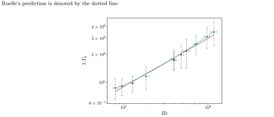
On the paper's own terms, the central discovery is that a single number — the Eulerian maximum Lyapunov exponent $\lambda$, averaged over many finite-time measurements — is a stable and quickly convergent descriptor of turbulence. Using direct numerical simulations with a fixed dissipation-rate forcing, the authors measure $\lambda$ by repeatedly perturbing a copy of the velocity field, letting the pair evolve for a short steptime $\Delta t$, and recording the logarithmic growth before renormalizing the difference to a small fixed amplitude $10^{-3}$. They find that $\lambda$ and its standard deviation $\sigma_\lambda$ barely change when the lattice size is varied at fixed viscosity, and barely change when $\Delta t$ is varied from values near the simulation timestep up to the direct-method limit. The exponent's autocorrelation time is about $0.5$ in simulation time units, roughly a tenth of the large-eddy turnover time, whereas energy decorrelates only after about two turnover times; hence a run of about ten turnover times gives converged Lyapunov statistics, while energy needs roughly a hundred. Fitting $\lambda T_0 = D\,\mathrm{Re}^\alpha$ with $T_0=L/U$ gives $\alpha=0.53\pm0.02$, agreeing with an earlier direct-method measurement; fitting with $T_{E0}=E/\varepsilon$ gives $\alpha_E=0.658\pm0.006$. The apparent conflict between the two exponents is explained by the Reynolds-dependent dimensionless dissipation rate $C_\varepsilon(\mathrm{Re}) = C_{\varepsilon,\infty} + C/\mathrm{Re}$, which converts $\alpha_E$ into an effective $\alpha\approx0.52$, and decaying-turbulence growth curves favor the $T_{E0}$-based functional form. In magnetohydrodynamic runs the robustness of $\lambda$ survives, but its Reynolds-number scaling is much shallower, $\alpha=0.14\pm0.02$.

Load-bearing premise

The paper assumes that averaging finite-time Lyapunov exponents, each obtained by renormalizing the perturbed field to a fixed tiny size at every short steptime, gives the true maximal Lyapunov exponent of the flow; it never tests whether changing that fixed size or extending the averaging time changes the result.

Editorial extensions

If this is right

A simulation run of roughly ten large-eddy turnover times is enough for converged Lyapunov statistics, while energy or Reynolds-number averages need about a hundred, so the Lyapunov exponent is a practical fast-converging flow diagnostic.
Because $\lambda$ and $\sigma_\lambda$ are nearly independent of the FTLE steptime down to very small values, short steptimes can be used to generate large samples at low computational cost.
Through the dimensional relation linking $\lambda$, $\mathrm{Re}$, and the large-eddy time, a measured $\lambda$ can serve as a fast proxy for Reynolds number or dissipation in homogeneous isotropic turbulence once calibration constants are known.
The effective exponent $\alpha$ in $\lambda T_0 = D\,\mathrm{Re}^\alpha$ is not a fixed universal number: it increases with Reynolds number and approaches $\alpha_E\approx0.66$ at high $\mathrm{Re}$, so the $\alpha=1/2$ dimensional prediction is not the fundamental scaling.
In MHD turbulence the Lyapunov exponent remains robust and steptime-stable, but its Reynolds-number power is much smaller ($\alpha=0.14\pm0.02$), so hydrodynamic calibrations should not be transferred to MHD flows.

Reading between the lines

Editorial extensions of the paper, not claims the author makes directly.

If the near-Gaussianity of the FTLE distribution is partly produced by the rapid renormalization injecting a fresh perturbation every steptime, then varying the perturbation amplitude or changing the forcing scheme should alter the distribution's shape and variance; this is a testable consequence the paper does not develop.
The observed excess fluctuation level $\sigma_\lambda/\lambda\approx0.2$ over the value propagated from $\mathrm{Re}$ and $T_0$ suggests either substantial finite-time and finite-perturbation effects or an attractor without a unique maximal exponent; distinguishing these would require measuring the full Lyapunov spectrum or varying $\delta_0$ systematically.
Because the decorrelation time $T_d$ is much longer than the steptime, the raw count of FTLE samples overstates the number of independent measurements; the effective independent-sample count is about $T_r/T_d$, so confidence intervals computed from raw counts alone are likely too optimistic.
The MHD results suggest that the exponent's Reynolds-number scaling tracks the existence of a single governing dissipative timescale; varying the magnetic Prandtl number in future simulations would test whether the shallow $\alpha=0.14$ scaling persists or shifts with the added magnetic timescales.

Share X Bluesky LinkedIn Reddit HN

Editorial analysis

A structured set of objections, weighed in public.

Desk editor's note, referee report, and a circularity audit.

Desk Editor's Note

read the letter

Colleague, here's my read of Ho et al. It's a solid, squarely empirical contribution to the Eulerian-chaos literature, not a breakthrough. What's genuinely new: a systematic demonstration that the mean and variance of FTLEs are insensitive to lattice size and to FTLE steptime, an approximate Gaussianity result for FTLE distributions, a run-time rule based on signal decorrelation, and a compact resolution of the alpha = 0.53 vs 0.64 discrepancy. The resolution is the best part: by using TE0 = E/epsilon and the Reynolds-dependent C_epsilon(Re) of McComb et al., the paper turns two apparently inconsistent scalings into one relation, and the predicted alpha ~ 0.52 matches the direct measurement. The decaying-turbulence test is a nice out-of-sample check, and it favors Eq. (21) without having been fit to that data, though the authors do allow a small post-hoc shift within error bars.

The main soft spot is real and the paper half-admits it: every quantitative claim—the exponents, the fluctuation scaling, the MHD comparison—passes through the FTLE estimator with delta0 fixed at 1e-3 and dt = 0.1, and there is no delta0 convergence study. Oseledets guarantees independence of the initial perturbation only in the delta0 -> 0, t -> infinity limits, and the authors cite Goldhirsch et al. for the finite-time, finite-perturbation dependence but never probe it. If the estimator carries a delta0-dependent bias, all fitted exponents shift together and the MHD contrast is suspect. One mitigating fact is that the hydrodynamic alpha = 0.53 matches the direct-method value from the same group [14], which is an independent estimator; that makes me think the mean is probably fine. But the fast-decorrelation and near-Gaussianity claims are explicitly conjectured by the authors to be possible artifacts of the perturbation method, so I would not treat those as flow physics until shown otherwise.

Other gaps are minor: steptime stability is shown for one simulation per fluid case; no code or data is shipped; the smallest lattice sizes are marginally resolved. None of that sinks the paper. The central scaling argument holds up; the missing delta0 test is a required revision, not a fatal flaw.

This one deserves a serious referee. It is useful for anyone running forced turbulence DNS who wants a practical run-time rule or a reconciliation of past Lyapunov-exponent scalings. I would send it to peer review with a request for a delta0 scan and, ideally, code/data release. I probably wouldn't cite it myself until the estimator sensitivity is closed.

Referee Report

4 major / 5 minor

Summary. The manuscript reports direct numerical simulations of forced homogeneous isotropic turbulence, plus a set of MHD runs, using the finite-time Lyapunov exponent (FTLE) method of Boffetta and Musacchio with perturbation amplitude δ0 = 10^-3 and steptime Δt = 0.1. It measures the mean Lyapunov exponent λ and its fluctuation σλ, fits λT0 = D Re^α (α = 0.53 ± 0.02) and λTE0 = DE Re^αE (αE = 0.658 ± 0.006), and attributes the difference between these exponents to the Reynolds-number-dependent dimensionless dissipation rate Cε(Re) of McComb et al. It further claims that FTLE histograms are approximately Gaussian while Reynolds-number histograms are not, that λ and σλ are insensitive to lattice size and steptime, that the Lyapunov signal decorrelates in about TE0/10 so that roughly 10TE0 of data suffice for converged statistics, that a decaying-turbulence test favors TE0 = E/ε as the relevant large-eddy timescale, and that MHD turbulence exhibits a much weaker scaling, α = 0.14 ± 0.02.

Significance. If the results hold, the paper provides a useful diagnostic: the Eulerian maximal Lyapunov exponent appears to be a comparatively cheap and stable statistical observable in both hydrodynamic and MHD turbulence. The explicit reconciliation of the earlier α = 0.53 versus 0.64 discrepancy through Cε(Re) is a concrete, checkable contribution, and the decaying-turbulence experiment is a genuine out-of-sample test because its constants were obtained from forced runs and then used to predict the growth of the difference field in an unforced flow. The autocorrelation analysis and the run-time rule Tr ≈ 100Td are practically valuable. The main weakness is that the FTLE estimator is not validated against the δ0→0 and t→∞ limits required by Oseledets theory, leaving the quantitative claims conditional.

major comments (4)

[II.A (Eqs. 11–12) and III.E (Fig. 12)] The central quantitative claims rest on the assumption that the mean FTLE, λ = ⟨λ̃⟩, is the true maximal Lyapunov exponent, but this is never validated. Oseledets' theorem guarantees independence of the initial perturbation only in the δ0→0 and t→∞ limits, and the paper explicitly concedes finite-perturbation and finite-time dependence [56]. Figure 12 varies the steptime Δt, not the perturbation amplitude δ0, which is fixed at 10^-3; decreasing Δt moves further from the t→∞ limit, and the agreement with the direct method is described only qualitatively in Section III.E. A δ0 scan (for example 10^-4 to 10^-5, ideally including a tangent-linear check) is needed to show that α, αE, σλ/λ ≈ 0.2, and the MHD comparison are properties of the flow rather than of the estimator. As written, a δ0-dependent bias would shift all fitted exponents and the hydrodynamic/MHD comparison together.
[III.A and IV (Figs. 14–17)] The claims that FTLEs are approximately Gaussian and that λ statistics decorrelate on a time Td ≈ 0.5 ≈ TE0/10 are flagged by the authors themselves as possibly being reset artifacts: Section III.A states that the near-Gaussianity 'could well be a consequence of the perturbation method', and Section IV states that the short self-correlation time 'might indicate that the perturbations introduced in the FTLE method have a relevant effect' on the measured signal. Because the fast-statistics result (run time of about 10TE0 rather than 100TE0) is one of the paper's main conclusions, it needs independent support. For example, the autocorrelation of a direct-method or tangent-linear signal could be compared, or Td could be shown to be insensitive to both Δt and δ0 over a wide range, rather than only noting that Td is larger than the steptime.
[III.D (Eqs. 19–24)] The reconciliation of α = 0.53 ± 0.02 with αE = 0.658 ± 0.006 is algebraically transparent, but the paper states 'strong agreement' between its simulation data and Eq. (19) without showing a plot or giving a quantitative comparison. Since Eq. (23) uses the constants Cε,∞ = 0.486 and C = 18.9 from [50] to predict ⟨α⟩exp ≈ 0.52, the reader needs to see the measured Cε(Re) values in the same figure or table to confirm that this correction is actually operating as claimed in the present runs.
[III.C and IV (Eq. 30, Table I)] The weighted least-squares fits in Sections III.C and III.D use σλ as a scatter measure, but the effective number of independent samples is not reported and the standard errors on the individual λ values are not given in Table I. If the fit weights are computed as σλ/√n without accounting for the autocorrelation (Td ≈ 0.5 and Δt = 0.1 imply several correlated samples per decorrelation time), the reported uncertainties on α and αE could be underestimated. Please state the weights used and the effective number of independent FTLE samples, or otherwise justify the error bars.

minor comments (5)

[IV (Figs. 14–17)] The autocorrelation lag is also denoted Δt, the same symbol as the FTLE steptime; although the text notes the distinction, using a separate symbol such as τlag would avoid confusion.
[III.A (Fig. 4)] The text reports n = 11863 FTLE samples from a run of 200T0, but with Δt = 0.1 and T0 = 2.43 from Table I this gives roughly 4860 samples; please clarify the run length or the steptime used for this figure.
[II.A (Eq. 14)] Equation (14) mixes ensemble-average and sample notations; it should be written as an explicit sample variance, for example σ²λ = (1/(n−1)) Σ (λ̃i − λ)², to make the estimator unambiguous.
[III.C (Eq. 17)] Equation (17) adds the two propagated errors linearly; for independent fluctuations the quadrature sum is the standard choice, and the linear sum should be justified as a conservative upper bound.
[V (Fig. 20)] The fit giving α = 0.14 ± 0.02 is not shown in Figure 20; please include the fitted line or state the fit procedure explicitly.

Circularity Check

0 steps flagged · score 0.0 of 10

No significant circularity: Lyapunov exponents are measured directly, the α resolution rests on an externally derived Cε(Re) relation, and the decaying-turbulence test is out-of-sample.

full rationale

The paper's central quantitative results are obtained from direct DNS measurements of finite-time Lyapunov exponents, not from an input-output equivalence. The claim that FTLEs are stable under steptime and lattice size is tested by varying those parameters explicitly (Figs. 5, 6, 12), not by construction. The resolution of the α discrepancy between [14] and [15] uses the dimensionless dissipation rate Cε(Re) from McComb et al. [50], which is derived independently from the von Kármán-Howarth equation and DNS, and whose constants do not involve the present λ data; the paper also states its own simulations are in strong agreement with [50]. The conversion between α and αE is a definitional relation (Eqs. 20, 22, 23), used as a consistency check rather than as a fitted-then-predicted quantity. The decaying turbulence prediction (Section III F) uses constants obtained from forced steady-state data to predict Ed(t) in a separate decaying run, which is an out-of-sample test. The main caveats—possible finite-perturbation and finite-time dependence of FTLEs, and the possibility that Gaussianity and fast decorrelation are artifacts of the perturbation method—are explicitly acknowledged by the authors, but acknowledging a methodological limitation is not circularity. The self-citations to [14] and [50] are prior measurements or derivations with independent content, not unverified postulates that the paper relies on to force its conclusions. No equation in the paper reduces to its own input by construction, and no fitted parameter is renamed as a prediction.

Assumptions & free parameters 12 free parameters · 8 assumptions · 0 invented entities

The main numerical claims rest on DNS data and empirical scaling fits. The fitted prefactors and exponents are listed; the key adopted input from prior literature is the Cepsilon(Re) relation from [50]. No new physical entities are introduced.

free parameters (12)

D in lambda T0 = D Re^alpha = 0.079 +/- 0.007
Prefactor fitted to 11 hydrodynamic DNS runs in Section III C, Figure 7.
alpha in lambda T0 = D Re^alpha = 0.53 +/- 0.02
Exponent fitted to the same data; it matches the direct-method value of [14] and is central to the discrepancy resolution.
D_E in lambda TE0 = D_E Re^alpha_E = 0.101 +/- 0.001
Prefactor fitted to the same data using TE0=E/epsilon, Figure 10.
alpha_E = 0.658 +/- 0.006
Exponent fitted to lambda TE0 versus Re; it matches the value of [15].
Cepsilon_infinity and C in Cepsilon(Re) = Cepsilon_infinity + C/Re = 0.486 +/- 0.006 and 18.9 +/- 1.3
Adopted from McComb et al. [50], same research group, and used in Eqs. (19)-(24) to convert between T0 and TE0 and to predict alpha.
gamma in sigma_lambda T0 proportional to Re^gamma = 0.62 +/- 0.05
Fit to fluctuation data, Figure 9.
gamma_E in sigma_lambda TE0 proportional to Re^gamma_E = 0.75 +/- 0.05
Fit using TE0; compared with the larger value reported in [15].
c1 in sigma_Re = c1 Re = 0.08 +/- 0.01
Linear fit for hydrodynamic Reynolds-number fluctuations, Figure 8.
c2 in sigma_lambda = c2 lambda = 0.20 +/- 0.02
Reported linear relation for hydrodynamic Lyapunov-exponent fluctuations.
c3 in sigma_Re = c3 Re (MHD) = 0.052 +/- 0.006
Linear fit for MHD Reynolds-number fluctuations, Figure 21.
A and B in linear fit lambda = A + B/tau (MHD) = A=0.19 +/- 0.02, B=0.037 +/- 0.004
Fit to the MHD Ruelle-relation plot, Figure 19.
delta0 perturbation amplitude = 10^-3
Fixed value in Eq. (11); chosen by hand and never varied, although the paper acknowledges finite-perturbation effects.

assumptions (8)

domain assumption The incompressible Navier-Stokes equations with negative-damping forcing (Eqs. 3-5) produce a statistically steady homogeneous isotropic turbulence state.
Used for all hydrodynamic DNS runs; the forcing sets epsilon approximately 0.1 and is from [51-53].
domain assumption The mean of finite-time Lyapunov exponents equals the maximal Lyapunov exponent despite finite-time and finite-perturbation effects.
Section II A invokes Oseledets [55] and notes finite-time dependence [56]; the paper averages over finite-time exponents.
domain assumption Time averages over the statistically steady state are representative of the ensemble (ergodicity).
Assumed throughout in computing lambda, sigma, Re, and T0 from finite simulation runs.
standard math The dimensional scaling lambda = D Re^alpha / T0 (Eq. 2) is the correct functional form, with alpha related to the Holder exponent.
Basis for the fits and for Ruelle's prediction; it is a dimensional-analysis ansatz, not derived in this paper.
domain assumption The dimensionless dissipation rate expansion Cepsilon(Re) = Cepsilon_infinity + C/Re from McComb et al. [50] applies to these simulations.
Crucial for converting between T0 and TE0 definitions in Section III D; the constants come from prior same-group DNS.
domain assumption In decaying turbulence, the perturbation grows as delta_u_{i+1} = delta_u_i exp(lambda_{i+1} delta_t) times |u_{i+1}|/|u_i|, with lambda varying slowly.
Equations (25)-(27) in Section III F; if lambda changes rapidly, the integrated prediction is invalid.
domain assumption Long time series can be partitioned into independent blocks of length equal to the decorrelation time Td, giving sigma_X/sigma = sqrt(Td/Tr).
The run-time rule Tr approximately 100 Td in Section IV relies on block independence and Gaussian standard-error behavior.
domain assumption For MHD, the combined velocity and magnetic field difference (Eq. 15) defines the appropriate Lyapunov exponent.
Section II A extends delta_t to include the magnetic field; no separate validation of this combined metric is provided.

how reviews work

0 comments

Cite this review

Pith. "Pith review of Fluctuations of Lyapunov Exponents in homogeneous and isotropic turbulence." pith.science (2026). https://pith.science/paper/EDILHWAR

@misc{pith2026190901177,
  author       = {Pith},
  title        = {Pith review of: Fluctuations of Lyapunov Exponents in homogeneous and isotropic turbulence},
  year         = {2026},
  howpublished = {\url{https://pith.science/paper/EDILHWAR}},
  note         = {Machine review of arXiv:1909.01177}
}

read the original abstract

In the context of the analysis of the chaotic properties of homogeneous and isotropic turbulence, direct numerical simulations are used to study the fluctuations of the finite time Lyapunov exponent (FTLE) and its relation to Reynolds number, lattice size and the choice of the steptime used to compute the Lyapunov exponents. The results show that using the FTLE method produces Lyapunov exponents that are remarkably stable under the variation of the steptime and lattice size. Furthermore, it reaches such stability faster than other characteristic quantities such as energy and dissipation rate. These results remain even if the steptime is made arbitrarily small. A discrepancy is also resolved between previous measurements of the dependence on the Reynolds number of the Lyapunov exponent. The signal produced by different variables in the steady state is analyzed and the self decorrelation time is used to determine the run time needed in the simulations to obtain proper statistics for each variable. Finally, a brief analysis on MHD flows is also presented, which shows that the Lyapunov exponent is still a robust measure in the simulations, although the Lyapunov exponent scaling with Reynolds number is significantly different from that of magnetically neutral hydrodynamic fluids.

Figures

Figures reproduced from arXiv: 1909.01177 by the authors.

**Figure 2.** FIG. 2. Normalized distributions of [PITH_FULL_IMAGE:figures/full_fig_p007_2.png] view at source ↗

**Figure 3.** FIG. 3. Histogram for the distribution of Re in a single run wi [PITH_FULL_IMAGE:figures/full_fig_p008_3.png] view at source ↗

Figures from the paper (19 more)

**Figure 4.** Figure 4: FIG. 4. Histogram for the distribution of [PITH_FULL_IMAGE:figures/full_fig_p008_4.png]

**Figure 5.** Figure 5: FIG. 5. Dependence of [PITH_FULL_IMAGE:figures/full_fig_p008_5.png]

**Figure 6.** Figure 6: FIG. 6. Dependence of Lyapunov exponent fluctuations [PITH_FULL_IMAGE:figures/full_fig_p009_6.png]

**Figure 7.** Figure 7: FIG. 7. (Color online) [PITH_FULL_IMAGE:figures/full_fig_p010_7.png]

**Figure 8.** Figure 8: FIG. 8 [PITH_FULL_IMAGE:figures/full_fig_p010_8.png]

**Figure 9.** Figure 9: FIG. 9. Data and linear fit to determine power law [PITH_FULL_IMAGE:figures/full_fig_p010_9.png]

**Figure 10.** Figure 10: FIG. 10. (Color online) [PITH_FULL_IMAGE:figures/full_fig_p012_10.png]

**Figure 11.** Figure 11: FIG. 11. (Color online) Data obtained for [PITH_FULL_IMAGE:figures/full_fig_p012_11.png]

**Figure 12.** Figure 12: shows the result of varying the steptime ∆t on the Lyapunov exponent and its fluctuations. The simulation has Re = 50. As can be seen in the Figure, the values of λ and σλ are remarkably stable even for very short steptimes using the FTLE method. Indeed, at the extrem…

**Figure 13.** Figure 13: FIG. 13. Different predictions of the functional form for [PITH_FULL_IMAGE:figures/full_fig_p014_13.png]

**Figure 14.** Figure 14: FIG. 14. Solid line shows complementary autocorrelation of [PITH_FULL_IMAGE:figures/full_fig_p015_14.png]

**Figure 15.** Figure 15: FIG. 15. Solid line shows complementary autocorrelation of [PITH_FULL_IMAGE:figures/full_fig_p016_15.png]

**Figure 16.** Figure 16: FIG. 16. Solid line shows complementary autocorrelation of [PITH_FULL_IMAGE:figures/full_fig_p016_16.png]

**Figure 17.** Figure 17: FIG. 17. Solid line shows complementary autocorrelation of [PITH_FULL_IMAGE:figures/full_fig_p017_17.png]

**Figure 18.** Figure 18: FIG. 18. Distributions of [PITH_FULL_IMAGE:figures/full_fig_p018_18.png]

**Figure 19.** Figure 19: FIG. 19 [PITH_FULL_IMAGE:figures/full_fig_p019_19.png]

**Figure 20.** Figure 20: FIG. 20 [PITH_FULL_IMAGE:figures/full_fig_p019_20.png]

**Figure 21.** Figure 21: FIG. 21. Distributions of [PITH_FULL_IMAGE:figures/full_fig_p020_21.png]

**Figure 22.** Figure 22: FIG. 22. Dependence of [PITH_FULL_IMAGE:figures/full_fig_p020_22.png]

Discussion (0). Continue with ORCID to comment.

Reference graph

Works this paper leans on

83 extracted references · 79 canonical work pages

[14]

00 0 . 05 0 . 10 0 . 15 0 . 20 0 . 25 0 . 30

work page
[56]

Haller and T

G. Haller and T. Sapsis, Chaos: An Interdiscip. J. Nonli nearSci. 21, 023115 (2011)

work page 2011
[50]

Biferale, G

L. Biferale, G. Boﬀetta, A. Celani, B. Devenish, A. Lano tte, and F. Toschi, Phys. Fluids 17, 115101 (2005)

work page 2005
[1]

0 1 . 2 1 . 4 1 . 6 1 . 8 2 . 0 2 . 2 2 . 4 ˜λ

work page
[2]

12 Probability density (a) 340 360 380 400 420 440 Re
[3]

025 Probability density (b) 850 900 950 1000 1050 1100 1150 Re
[4]

008 Probability density (c) FIG. 1. Normalized distributions of Re for three simulation s: (a) N = 128 and ν = 0 .01 , (b) N = 256 and ν = 0 .0018, (c) N = 512 and ν = 0.0008. The black line represents the Gaussian function with m ean and variance given by the distribution. B. Dependence of λ and Re on lattice size We look at the dependence of the Lyapuno...

work page
[5]

25 0 . 30 0 . 35 0 . 40 0 . 45 0 . 50 ˜λ 0 1 2 3 4 5 6 7Probability density (a)

work page

Show all 83 references

[6]

6 0 . 8 1 . 0 1 . 2 1 . 4 ˜λ
[7]

0 Probability density (b)
[8]

Leith, J

C. Leith, J. Atmospheric Sci. 28, 145 (1971)

1971
[9]

0 Probability density (c) FIG. 2. Normalized distributions of ˜λ for three simulations: (a) N = 128 and ν = 0 .01, (b) N = 256 and ν = 0 .0018, (c) N = 512 and ν = 0.0008. The black line represents the Gaussian function with m ean and variance given by the distribution. on the...
[10]

08 Probability density FIG. 3. Histogram for the distribution of Re in a single run wi th measurement time of approximately 500 T0. The solid black line represents the Gaussian function with mean and varianc e corresponding to the data sample
[11]

25 0 . 30 0 . 35 0 . 40 0 . 45 ˜λ 0 1 2 3 4 5 6 7 8Probability density FIG. 4. Histogram for the distribution of ˜λ in a single run with N = 128 and ν = 0.01, obtaining a large sample of n = 11863. The solid black line represents the Gaussian function with v ariance and mean g...
[12]

44 λ FIG. 5. Dependence of λ on lattice size N , diﬀerent shapes represent diﬀerent initial seeds. 9 25 26 27 28 29 N
[13]

15 σλ T0 FIG. 6. Dependence of Lyapunov exponent ﬂuctuations σλ T0 vs. N , diﬀerent shapes represent diﬀerent seeds for the initial random ﬁeld for each lattice size N 3 ν ε Re λ σ λ T0 TE0 τ k maxη 1283 0.0100 0.096 80.0 0.359 0.057 2.43 5.17 0.323 2.39 1283 0.0080 0.097 96.0...

1935
[15]

00 0 . 05 0 . 10 0 . 15 0 . 20 0 . 25 0 . 30 ∆ t
[16]

0575 σλ FIG. 12. Dependence of λ and σλ on the steptime ∆ t. Figure 12 shows the result of varying the steptime ∆ t on the Lyapunov exponent and its ﬂuctuations. The simulation has Re = 50. As can be seen in the Figure, the values of λ and σλ are remarkably stable even for ver...
[17]

15 0 . 20 0 . 25 0 . 30 0 . 35 0 . 40 ˜λ 0 2 4 6 8Probability density (a) 75 80 85 90 95 Re
[18]

07 probability density (b) FIG. 18. Distributions of λ and Re for the MHD case for one simulation. time and length scales than magnetically neutral ﬂows, given that fo r each velocity ﬁeld length and time scale, there is a corresponding time or length scale for the magnetic ﬁe...
[19]

50 λ FIG. 19. λ vs τ − 1 (the inverse of Kolmogorov time τ = (ν/ǫ)1/ 2) and linear ﬁt represented by the solid red line. 102 103 Re 100 6 × 10− 1 λT 0 FIG. 20. λT0 vs. Re using the FTLE method in a MHD ﬂuid We now compare the dependence of σλ on λ and σRe on Re, as was done fo...
[20]

1 0 . 2 0 . 3 0 . 4 0 . 5 0 . 6
[21]

1 0 . 2 0 . 3 0 . 4 0 . 5 0 . 6 ∆ t
[22]

0550 σλ FIG. 22. Dependence of λ and σλ on the steptime ∆ t of the FTLE method for MHD ﬂows. such as Reynolds number, lattice size and steptime in the FTLE proce dure. There are four main results which we may take from the analysis done in this paper. The ﬁrst is that the FTLE...
[23]

Ruelle and F

D. Ruelle and F. Takens, Comm. Math. Phys. 20, 167 (1971)

1971
[24]

Deissler, Phys

R. Deissler, Phys. Fluids 29, 1453 (1986)

1986
[25]

E. N. Lorenz, J. Atmospheric Sci. 20, 130 (1963)

1963
[26]

Yoden and M

S. Yoden and M. Nomura, J. Atmospheric Sci. 50, 1531 (1993)

1993
[27]

Masuoka, Y

T. Masuoka, Y. Takatsu, and T. Inoue, Microscale Thermop hys. Eng. 6, 347 (2003)

2003
[28]

Musker, AIAA J

A. Musker, AIAA J. 17, 655 (1979)

1979
[29]

D. C. Poirel and S. J. Price, AIAA J. 39, 1960 (2001)

2001
[30]

Vannitsem, Chaos: An Interdiscip

S. Vannitsem, Chaos: An Interdiscip. J. NonlinearSci. 27, 032101 (2017)

2017
[31]

Leith and R

C. Leith and R. Kraichnan, J. Atmospheric Sci. 29, 1041 (1972)

1972
[32]

Aurell, G

E. Aurell, G. Boﬀetta, A. Crisanti, G. Paladin, and A. Vu lpiani, J. Phys. A: Math. Gen. 30, 1 (1997)

1997
[33]

Kurths and H

J. Kurths and H. Herzel, Sol. Phys. 107, 39 (1986)

1986
[34]

Grappin, J

R. Grappin, J. Leorat, and A. Pouquet, J. de Physique 47, 1127 (1986)

1986
[35]

Huang, W

W. Huang, W. Ding, D. Feng, and C. Yu, Phys. Rev. E 50, 1062 (1994)

1994
[36]

Berera and R

A. Berera and R. D. J. G. Ho, Phys. Rev. Lett. 120, 024101 (2018)

2018
[37]

Boﬀetta and S

G. Boﬀetta and S. Musacchio, Phys. Rev. Lett. 119, 054102 (2017). 22

2017
[38]

Mohan, N

P. Mohan, N. Fitzsimmons, and R. D. Moser, Phys. Rev. Flu ids 2, 114606 (2017)

2017
[39]

R. D. Ho, A. Berera, and D. Clark, Phys. Plasmas 26, 042303 (2019)

2019
[40]

Nastac, J

G. Nastac, J. W. Labahn, L. Magri, and M. Ihme, Phys. Rev. Fluids 2, 094606 (2017)

2017
[41]

Mukherjee, J

S. Mukherjee, J. Schalkwijk, and H. J. Jonker, J. Atmosp heric Sci. 73, 2715 (2016)

2016
[42]

Y. C. Li, R. D. Ho, A. Berera, and Z. Feng, arXiv preprint a rXiv:1908.04838 (2019)

2019 arXiv
[43]

Boﬀetta, A

G. Boﬀetta, A. Celani, A. Crisanti, and A. Vulpiani, Phy s. Fluids 9, 724 (1997)

1997
[44]

Boﬀetta and S

G. Boﬀetta and S. Musacchio, Phys. Fluids 13, 1060 (2001)

2001
[45]

M´ etais and M

O. M´ etais and M. Lesieur, J. Atmospheric Sci. 43, 857 (1986)

1986
[46]

Crisanti, M

A. Crisanti, M. Jensen, A. Vulpiani, and G. Paladin, Phy s. Rev. Lett. 70, 166 (1993)

1993
[47]

Yamada and Y

M. Yamada and Y. Saiki, Nonlinear Process. Geophys. 14, 631 (2007)

2007
[48]

de Divitiis, Adv.Math

N. de Divitiis, Adv.Math. Phys. 2018 (2018)

2018
[49]

Lapeyre, Chaos: An Interdiscip

G. Lapeyre, Chaos: An Interdiscip. J. NonlinearSci. 12, 688 (2002)

2002
[51]

Biferale, G

L. Biferale, G. Boﬀetta, A. Celani, B. Devenish, A. Lano tte, and F. Toschi, Phys. Fluids 17, 111701 (2005)

2005
[52]

Ishihara and Y

T. Ishihara and Y. Kaneda, in Statistical Theories and Computational Approaches to Turb ulence (Springer, 2003) pp. 177–188

2003
[53]

H. Guo, W. He, T. Peterka, H.-W. Shen, S. M. Collis, and J. J. Helmus, IEEE Trans. Vis. Comput. Graph. 22, 1672 (2016)

2016
[54]

Garaboa-Paz, J

D. Garaboa-Paz, J. Eiras-Barca, and V. P´ erez-Mu˜ nuzuri, Earth Syst. Dyn. 8, 865 (2017)

2017
[55]

d’Ovidio, V

F. d’Ovidio, V. Fern´ andez, E. Hern´ andez-Garc ´ ıa, and C. L´ opez, Geophys. Res. Lett. 31 (2004)

2004
[57]

Haller, Annu

G. Haller, Annu. Rev. Fluid Mech. 47, 137 (2015)

2015
[58]

E. R. Abraham and M. M. Bowen, Chaos: An Interdiscip. J. N onlinearSci. 12, 373 (2002)

2002
[59]

A. C.-L. Chian, S. S. Silva, E. L. Rempel, M. Goˇ si´ c, L. R . B. Rubio, R. A. Miranda, and I. S. Requerey, arXiv:1904.084 72 (2019)

2019
[60]

Rempel, A.-L

E. Rempel, A.-L. Chian, F. J. Beron-Vera, S. Szanyi, and G. Haller, Mon. Notices Royal Astron. Soc. 466, L108 (2016)

2016
[61]

A. C.-L. Chian, E. L. Rempel, G. Aulanier, B. Schmieder, S. C. Shadden, B. T. Welsch, and A. R. Yeates, The Astrophys. J 786, 51 (2014)

2014
[62]

Tang, C.-C

J.-N. Tang, C.-C. Tseng, and N.-F. Wang, Acta Mech. Sin. 28, 612 (2012)

2012
[63]

T. S. Pedersen, P. K. Michelsen, and J. J. Rasmussen, Phy s. Plasmas 3, 2939 (1996)

1996
[64]

Padberg, T

K. Padberg, T. Hauﬀ, F. Jenko, and O. Junge, New J. Phys. 9, 400 (2007)

2007
[65]

Falessi, F

M. Falessi, F. Pegoraro, and T. Schep, J. Plasma Phys. 81 (2015)

2015
[66]

Misguich, R

J. Misguich, R. Balescu, H. Pecsell, T. Mikkelsen, S. La rsen, and Q. Xiaoming, Plasma Phys. Control. Fusion 29, 825 (1987)

1987
[67]

S. C. Shadden, F. Lekien, and J. E. Marsden, Phys. D: Nonl inear Phenom. 212, 271 (2005)

2005
[68]

P. L. Johnson and C. Meneveau, Phys. Fluids 27, 085110 (2015)

2015
[69]

Shimada and T

I. Shimada and T. Nagashima, Prog. Theor. Exp. Phys. 61, 1605 (1979)

1979
[70]

0 72 . 5 75 . 0 77 . 5 80 . 0 82 . 5 85 . 0 87 . 5 Re
[71]

Ruelle, Phys

D. Ruelle, Phys. Lett. A 72, 81 (1979)

1979
[72]

A. N. Kolmogorov, Proc. Royal Soc. Lond. A 434, 15 (1991)

1991
[73]

W. D. Mccomb, A. Berera, S. R. Yoﬀe, and M. F. Linkmann, Ph ys. Rev. E 91 (2015)

2015
[74]

Machiels, Phys

L. Machiels, Phys. Rev. Lett. 79, 3411 (1997)

1997
[75]

S. R. Yoﬀe, arXiv:1306.3408 (2013)

2013 arXiv
[76]

S. L. Brunton and C. W. Rowley, Chaos: An Interdiscip. J. NonlinearSci. 20, 017503 (2010)

2010
[77]

V. I. Oseledets, Trans. Moscow Mater. Soc. 19, 179 (1968)

1968
[78]

Goldhirsch, P.-L

I. Goldhirsch, P.-L. Sulem, and S. A. Orszag, Phys. D: No nlinear Phenom. 27, 311 (1987)

1987
[79]

G. I. Taylor, Proc. Royal Soc. Lond. A 151, 421 (1935)

1935
[80]

C. R. Doering and P. Constantin, Phys. Rev. E 49, 4087 (1994)

1994
[81]

K. R. Sreenivasan, Phys. Fluids 10, 528 (1998)

1998
[82]

Gotoh, D

T. Gotoh, D. Fukayama, and T. Nakano, Phys. Fluids 14, 1065 (2002)

2002
[83]

M. F. Linkmann and A. Morozov, Phys. Rev. Lett. 115, 134502 (2015)

2015

Pith tools

Reviewed August 14, 2026 · model on record in the stance chip above.

[1] [14]

00 0 . 05 0 . 10 0 . 15 0 . 20 0 . 25 0 . 30

work page

[2] [56]

Haller and T

G. Haller and T. Sapsis, Chaos: An Interdiscip. J. Nonli nearSci. 21, 023115 (2011)

work page 2011

[3] [50]

Biferale, G

L. Biferale, G. Boﬀetta, A. Celani, B. Devenish, A. Lano tte, and F. Toschi, Phys. Fluids 17, 115101 (2005)

work page 2005

[4] [1]

0 1 . 2 1 . 4 1 . 6 1 . 8 2 . 0 2 . 2 2 . 4 ˜λ

work page

[5] [2]

12 Probability density (a) 340 360 380 400 420 440 Re

[6] [3]

025 Probability density (b) 850 900 950 1000 1050 1100 1150 Re

[7] [4]

008 Probability density (c) FIG. 1. Normalized distributions of Re for three simulation s: (a) N = 128 and ν = 0 .01 , (b) N = 256 and ν = 0 .0018, (c) N = 512 and ν = 0.0008. The black line represents the Gaussian function with m ean and variance given by the distribution. B. Dependence of λ and Re on lattice size We look at the dependence of the Lyapuno...

work page

[8] [5]

25 0 . 30 0 . 35 0 . 40 0 . 45 0 . 50 ˜λ 0 1 2 3 4 5 6 7Probability density (a)

work page