A PDE model for unidirectional flows: stationary profiles and asymptotic behaviour
Pith reviewed 2026-05-24 14:13 UTC · model grok-4.3
The pith
Stationary profiles in a convection-diffusion model for unidirectional flows have boundary layers whose location and shape are fixed by inflow conditions, outflow conditions, and domain geometry.
A machine-rendered reading of the paper's core claim, the machinery that carries it, and where it could break.
Core claim
The location and shape of boundary layers in the stationary profiles can be related to the inflow and outflow conditions as well as the shape of the domain using geometric singular perturbation theory.
What carries the argument
Geometric singular perturbation theory applied to the reduced slow-fast system arising from the stationary convection-diffusion equation, which identifies the asymptotic layer locations and profiles.
If this is right
- Boundary layers form near the entrance or exit according to whether flow enters or leaves at that boundary.
- Changes in domain shape alter the existence or thickness of layers in the stationary profiles.
- The asymptotic analysis yields explicit descriptions of the profiles outside the layers.
- Numerical experiments reproduce the layer structures predicted by the geometric singular perturbation analysis.
Where Pith is reading between the lines
- The same reduction and layer analysis could be applied to time-dependent versions of the model to track how layers evolve.
- The approach may connect to other convection-dominated problems on bounded domains where inflow and outflow data control interior structure.
- Predictions for layer placement could be checked against laboratory experiments with controlled pedestrian or fluid flows matching the boundary data.
Load-bearing premise
The stationary problem and chosen boundary conditions reduce to a slow-fast system that has no additional singularities introduced by the domain geometry.
What would settle it
A computed stationary profile in a concrete domain whose boundary-layer locations or thicknesses fail to match the positions predicted from the inflow, outflow, and geometry would falsify the claimed relation.
Figures


read the original abstract
In this paper, we investigate the stationary profiles of a convection-diffusion model for unidirectional pedestrian flows in domains with a single entrance and exit. The inflow and outflow conditions at both the entrance and exit as well as the shape of the domain have a strong influence on the structure of stationary profiles, in particular on the formation of boundary layers. We are able to relate the location and shape of these layers to the inflow and outflow conditions as well as the shape of the domain using geometric singular perturbation theory. Furthermore, we confirm and exemplify our analytical results by means of computational experiments.
Editorial analysis
A structured set of objections, weighed in public.
Referee Report
Summary. The paper investigates stationary profiles of a convection-diffusion PDE model for unidirectional pedestrian flows in domains with a single entrance and exit. It claims that the location and shape of boundary layers can be related to the inflow/outflow conditions and domain shape via geometric singular perturbation theory (GSPT), with the analytical findings confirmed by numerical experiments.
Significance. If the GSPT reduction holds, the work provides a useful analytical framework for understanding how geometry and boundary data control layer formation in convection-dominated flows, with direct relevance to crowd dynamics modeling. The explicit use of GSPT (normal hyperbolicity, Fenichel theory) together with computational validation is a strength, as is the focus on falsifiable predictions for layer location.
major comments (1)
- [GSPT reduction / coordinate transformation section] The central claim requires that a coordinate change adapted to general domain geometry reduces the stationary convection-diffusion equation to a slow-fast system to which standard GSPT applies without obstruction. The Laplacian in curvilinear coordinates produces first-order curvature terms that remain O(1) as the diffusion parameter tends to zero; these can destroy scale separation or normal hyperbolicity. The manuscript must explicitly derive the transformed system (likely in §3 or the GSPT section) and verify that curvature contributions either vanish or are absorbed into the fast/slow scaling without creating additional singularities at inflow/outflow boundaries.
minor comments (2)
- [Model formulation] Clarify the precise form of the inflow/outflow boundary conditions (Dirichlet, Neumann, or Robin) and confirm they are compatible with the reduced flow on the slow manifold.
- [Computational experiments] In the numerical section, report the range of the small parameter used and any mesh refinement or error indicators that confirm the observed layers are not numerical artifacts.
Simulated Author's Rebuttal
We thank the referee for the careful and constructive report. The single major comment is addressed below; we will revise the manuscript to incorporate an explicit derivation as requested.
read point-by-point responses
-
Referee: The central claim requires that a coordinate change adapted to general domain geometry reduces the stationary convection-diffusion equation to a slow-fast system to which standard GSPT applies without obstruction. The Laplacian in curvilinear coordinates produces first-order curvature terms that remain O(1) as the diffusion parameter tends to zero; these can destroy scale separation or normal hyperbolicity. The manuscript must explicitly derive the transformed system (likely in §3 or the GSPT section) and verify that curvature contributions either vanish or are absorbed into the fast/slow scaling without creating additional singularities at inflow/outflow boundaries.
Authors: We agree that the transformed system must be derived explicitly to confirm applicability of GSPT. In the revised manuscript we will add a dedicated subsection (in §3) that performs the curvilinear coordinate change for a general domain with a single entrance/exit. The derivation will show that the first-order curvature terms arising from the Laplacian enter the slow equation as O(1) corrections that are absorbed into the reduced slow flow without destroying normal hyperbolicity of the critical manifold or introducing singularities at the inflow/outflow boundaries; the fast scaling remains dominant in the layer regions. This will make the application of Fenichel theory fully rigorous and falsifiable as claimed. revision: yes
Circularity Check
No circularity: derivation applies standard external GSPT to the PDE system
full rationale
The paper derives stationary profile structure and boundary layer location/shape from the convection-diffusion PDE by reducing to a slow-fast system and invoking geometric singular perturbation theory (normal hyperbolicity, Fenichel theory). This is an external, independently established mathematical technique whose validity does not depend on the present paper's fitted values or self-referential definitions. No equations in the abstract or described chain reduce a claimed prediction to a fitted parameter or to a prior self-citation that itself assumes the target result. The domain-geometry dependence enters through coordinate changes whose validity is checked within the GSPT framework rather than by construction.
Axiom & Free-Parameter Ledger
axioms (1)
- domain assumption The convection-diffusion system admits a slow-fast decomposition suitable for geometric singular perturbation analysis under the given boundary conditions.
Reference graph
Works this paper leans on
- [1]
- [2]
-
[3]
M. Burger and J.-F. Pietschmann. Flow characteristics in a crowded transport model. Non- linearity, 29(11):3528–3550, 2016
work page 2016
- [4]
-
[5]
E. Cristiani, B. Piccoli, and A. Tosin. Multiscale modeling of pedestrian dynamics, volume 12. Springer, 2014
work page 2014
- [6]
-
[7]
G. Giacomin and J. L. Lebowitz. Phase segregation dynamics in particle systems with long range interactions. I. Macroscopic limits. J. Statist. Phys. , 87(1-2):37–61, 1997
work page 1997
-
[8]
S. N. Gomes, A. M. Stuart, and M.-T. Wolfram. Parameter estimation for macroscopic pedestrian dynamics models from microscopic data. SIAM Journal on Applied Mathematics , 79(4):1475–1500, 2019
work page 2019
-
[9]
B. D. Greenshields, J. T. Thompson, H. C. Dickinson, and R. S. Swinton. The photographic method of studying traffic behavior. In Highway Research Board Proceedings, volume 13, 1934
work page 1934
-
[10]
F. A. Haight. Mathematical theories of traffic flow. Academic Press, New York-London, 1963
work page 1963
- [11]
-
[12]
D. Helbing and P. Molnar. Social force model for pedestrian dynamics. Physical review E , 51(5):4282, 1995
work page 1995
- [13]
-
[14]
C. K. R. T. Jones. Geometric singular perturbation theory. In Dynamical Systems , pages 44–118. Springer Berlin Heidelberg, 1995
work page 1995
-
[15]
C. Kuehn. Multiple Time Scale Dynamics . Springer International Publishing, 2015
work page 2015
-
[16]
M. J. Lighthill and G. B. Whitham. On kinematic waves II. A theory of traffic flow on long crowded roads. Proceedings of the Royal Society of London. Series A. Mathematical and Physical Sciences, 229(1178):317–345, 1955
work page 1955
-
[17]
A. Logg, K.-A. Mardal, G. N. Wells, et al. Automated Solution of Differential Equations by the Finite Element Method . Springer, 2012
work page 2012
-
[18]
A. Logg and G. N. Wells. Dolfin: Automated finite element computing. ACM Transactions on Mathematical Software, 37(2), 2010
work page 2010
-
[19]
B. Piccoli and A. Tosin. Pedestrian flows in bounded domains with obstacles. Continuum Mechanics and Thermodynamics, 21(2):85–107, 2009
work page 2009
-
[20]
P. I. Richards. Shock waves on the highway. Operations research, 4(1):42–51, 1956
work page 1956
-
[21]
A. Seyfried, B. Steffen, W. Klingsch, T. Lippert, and M. Boltes. The fundamental diagram of pedestrian movement revisited — empirical results and modelling. In A. Schadschneider, T. P¨ oschel, R. K¨ uhne, M. Schreckenberg, and D. E. Wolf, editors, Traffic and Granular Flow’05, pages 305–314, Berlin, Heidelberg, 2007. Springer Berlin Heidelberg
work page 2007
-
[22]
P. Szmolyan and M. Wechselberger. Canards in R3. Journal of Differential Equations , 177(2):419–453, 2001
work page 2001
-
[23]
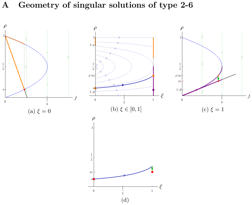
P. Szmolyan and M. Wechselberger. Relaxation oscillations in R3. Journal of Differential Equations, 200(1):69–104, 2004. 28 A Geometry of singular solutions of type 2-6 (a) ξ = 0 (b) ξ∈ [0, 1] (c) ξ = 1 (d) Figure 15: Schematic representation of a singular solution of type 2. (a) Boundary conditions at ξ = 0 in ( j, ρ)-space: the orange line is L, while th...
work page 2004
-
[24]
(blue curve). The orange lines are the projection of L (at ξ = 0) and L+ (at ξ = 1) on C0, while the purple one represents the projection of R− onC0 at ξ = 1. The orange dots correspond to l (at ξ = 0) and l1 (at ξ = 1), while the purple dot corresponds to r. (c) Here, we consider ξ = 1 in ( j, ρ)-space. The red dot corresponds to p1, while the purple lin...
-
[25]
(blue curve). The orange lines are the projection of L (at ξ = 0) andL+ (at ξ = 1) onC0, while the purple one represents the projection of R− onC0 at ξ = 1. The orange dots correspond to l (at ξ = 0) and l1 (at ξ = 1), while the purple dot corresponds to r. (c) Here, we consider ξ = 1 in (j, ρ)-space. The red dot corresponds to p1, while the purple line a...
-
[26]
The respective bifurcation diagram is shown in Figure 20
The solutions allow us to compute explicit profiles for all combinations of α and β (extending the results in [3]). The respective bifurcation diagram is shown in Figure 20. The constant ξ can be computed from the Figure 20: Phase diagram illustrating the stationary profiles for different inflow and outflow pa- rameters α and β, along with the respective expre...
discussion (0)
Sign in with ORCID, Apple, or X to comment. Anyone can read and Pith papers without signing in.