pith. sign in

arxiv: 2312.12396 · v2 · submitted 2023-12-09 · 📊 stat.ME

A Bayesian time-varying random partition model for large spatio-temporal datasets

Pith reviewed 2026-05-24 05:08 UTC · model grok-4.3

classification 📊 stat.ME
keywords Bayesian clusteringspatio-temporal datarandom partition priortime-varying regimesspatial proximitychangepointsmobile phone usageMilan
0
0 comments X

The pith

A Bayesian model with a novel random partition prior clusters spatio-temporal data into time-varying spatial groups based on proximity.

A machine-rendered reading of the paper's core claim, the machinery that carries it, and where it could break.

The paper proposes a semi-parametric hierarchical Bayesian model for large spatio-temporal areal datasets that performs model-based clustering varying over both space and time. It defines regimes for different periods such as work versus night hours and weekdays versus weekends, with changes handled through temporal changepoint components that permit different hierarchical structures at different times. The central innovation is a random partition prior that builds in spatial features by encouraging co-clustering of nearby areas according to a given neighboring structure. Motivated by mobile phone usage data from the Milan metropolitan area, the model aims to recover population patterns that shift across these regimes. If the approach works, it supplies a flexible way to analyze correlated time series across space without assuming fixed clusters throughout the observation period.

Core claim

The central claim is that the proposed semi-parametric hierarchical Bayesian model, which incorporates temporal changepoint components for regime shifts and a novel random partition prior that encourages co-clustering based on areal proximity, enables joint time-varying and spatial model-based clustering for large spatio-temporal datasets.

What carries the argument

The novel random partition prior that incorporates the desired spatial features and encourages co-clustering based on areal proximity, used inside a hierarchical Bayesian setup with temporal changepoints occurring within fixed time windows.

If this is right

  • The model identifies distinct spatial clusters of usage patterns that differ across work hours, nights, weekdays, and weekends.
  • It supports analysis of large datasets via its semi-parametric structure and Bayesian uncertainty quantification.
  • Simulation studies allow direct assessment of the prior's ability to recover known partitions under controlled spatial and temporal conditions.
  • The Milan application produces clusters that reflect changing population movement patterns across the metropolitan area.

Where Pith is reading between the lines

These are editorial extensions of the paper, not claims the author makes directly.

  • The same prior structure could be tested on other areal datasets such as traffic counts or pollution measurements to check whether proximity-based clustering generalizes.
  • Allowing the changepoint windows themselves to be estimated from data rather than fixed in advance would remove one modeling restriction.
  • If the recovered clusters align with known urban zones, they could support downstream tasks such as resource allocation without additional spatial modeling.
  • The framework might be combined with non-Bayesian clustering methods for faster initial exploration before full posterior sampling.

Load-bearing premise

The approach assumes a known neighbouring structure for the spatial correlation and that changepoints occur within fixed time windows over the day.

What would settle it

Simulation experiments in which the true spatial partitions and temporal regimes are known in advance but the model recovers them with low accuracy, or application to the Milan mobile phone data that yields clusters unrelated to observable usage differences between work, night, and weekend periods.

Figures

Figures reproduced from arXiv: 2312.12396 by Alessandra Guglielmi, Andrea Cremaschi, Annalisa Cadonna, Fernando Andr\'es Quintana, Giulio Beltramin.

Figure 1
Figure 1. Figure 1: Data recorded on Wednesday March 18th 2009, at noon. The grey areas corresponds to [PITH_FULL_IMAGE:figures/full_fig_p008_1.png] view at source ↗
Figure 2
Figure 2. Figure 2: Standardized log-Erlang numbers for data recorded over time at 10 randomly selected locations. that a zero Erlang number does not mean zero activity, but that this fell below a certain detection threshold. Then, the log-transformed data are standardized to have mean 0 and standard deviation 1. 9 [PITH_FULL_IMAGE:figures/full_fig_p009_2.png] view at source ↗
Figure 3
Figure 3. Figure 3: Distribution of the number of clusters Kn under the prior for ρ as in Hegarty and Barry (2008), for different values of ξ. reflect changes appearing through time, allowing for a regime-specific prior distribution for the partition of areas. Firstly, we elaborate on the concept of regime and its relationship with the clustering of observations. A regime rt at time t ∈ [T] is associated to a partition of the… view at source ↗
Figure 4
Figure 4. Figure 4: Distribution of the number of clusters Kn under the our prior for ρ (see (5)), which includes a DP term, for different values of ξ. The mass parameter κ is fixed to 1. time points over the time period under study, we must permit the same partition ρrt to exist at these time points, effectively exploiting the division of the set [T] of time points into M ≥ nR non-overlapping sets. For instance, in our appli… view at source ↗
Figure 5
Figure 5. Figure 5: Illustration of the regime scheme in the case under study. Throughout the time interval, the [PITH_FULL_IMAGE:figures/full_fig_p020_5.png] view at source ↗
Figure 6
Figure 6. Figure 6: Telecom data. Posterior estimate of the random partition [PITH_FULL_IMAGE:figures/full_fig_p025_6.png] view at source ↗
Figure 7
Figure 7. Figure 7: Telecom data. Posterior estimate of the random partition [PITH_FULL_IMAGE:figures/full_fig_p026_7.png] view at source ↗
Figure 8
Figure 8. Figure 8: Telecom data. Observed trajectories colored according to the estimated VI partition. [PITH_FULL_IMAGE:figures/full_fig_p029_8.png] view at source ↗
Figure 9
Figure 9. Figure 9: Telecom data. Posterior distribution of the Rand Index between [PITH_FULL_IMAGE:figures/full_fig_p030_9.png] view at source ↗
Figure 10
Figure 10. Figure 10: Telecom data. Posterior mean and 95% credible interval for [PITH_FULL_IMAGE:figures/full_fig_p031_10.png] view at source ↗
Figure 11
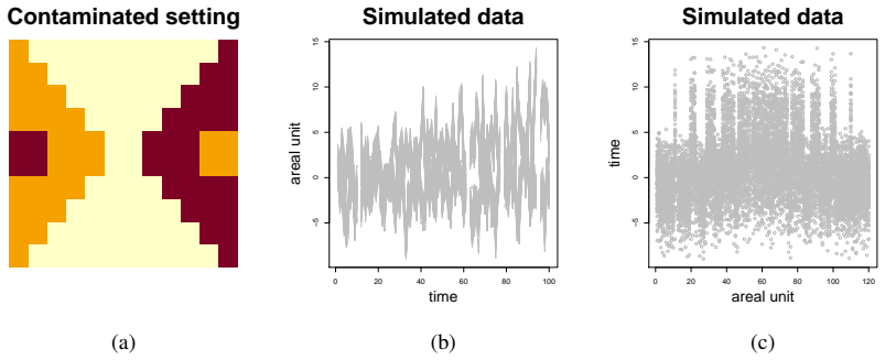
Figure 11. Figure 11: Simulated data (nR = 1). (a) The original clustering of the data shows areal contamina￾tion. (b) Plot of the trajectories for each areal units. (c) Plot of the data for each time point as function of the areal units. the simulations, despite convergence. This behavior seems to reflect the identifiability issues already pointed out in Section 3.4. We proceed the investigation by looking at the posterior es… view at source ↗
Figure 12
Figure 12. Figure 12: Simulated data (nR = 1). (a,b,c) Traceplots of the parameters τ 2 , σ 2 ϵ and ζ. The value of the parameters used to simulate the data is indicated as a red horizontal line. (d) Posterior mean of the areal random effects (truth in red). 44 [PITH_FULL_IMAGE:figures/full_fig_p044_12.png] view at source ↗
Figure 13
Figure 13. Figure 13: Simulated data (nR = 1). Posterior estimates of the partition of the areal units obtained by minimizing the Variation of Information loss function. 45 [PITH_FULL_IMAGE:figures/full_fig_p045_13.png] view at source ↗
Figure 14
Figure 14. Figure 14: Simulated data (nR = 1). (a) The original clustering of the data shows areal contamina￾tion. (b) Plot of the trajectories for each areal units. (c) Plot of the data for each time point as function of the areal units. Single regime with contaminated clusters and missing data We present another simulation example with one regime only (nR = 1). As in the previous example, a grid of size 12 × 10 is used (I = … view at source ↗
Figure 15
Figure 15. Figure 15: Simulated data (nR = 1). (a,b,c) Traceplots of the parameters τ 2 , σ 2 ϵ and ζ. The value of the parameters used to simulate the data is indicated as a red horizontal line. (d) Posterior mean of the areal random effects (truth in red). 48 [PITH_FULL_IMAGE:figures/full_fig_p048_15.png] view at source ↗
Figure 16
Figure 16. Figure 16: Simulated data (nR = 1). Posterior estimates of the partition of the areal units obtained by minimizing the Variation of Information loss function. 49 [PITH_FULL_IMAGE:figures/full_fig_p049_16.png] view at source ↗
Figure 17
Figure 17. Figure 17: Simulated data (nR = 1). Traceplots of the imputed missing value at location/time (i, t) = (94, 4) under different model specifications. 50 [PITH_FULL_IMAGE:figures/full_fig_p050_17.png] view at source ↗
Figure 18
Figure 18. Figure 18: Simulated data (nR = 1). Traceplots of the imputed missing value at location/time (i, t) = (24, 50) under different model specifications. This areal unit was missing observations at all time points. 51 [PITH_FULL_IMAGE:figures/full_fig_p051_18.png] view at source ↗
Figure 19
Figure 19. Figure 19: Simulated data (nR = 1). Traceplots of the imputed missing value at location/time (i, t) = (10, 21) under different model specifications. This time point was missing observations at all areal units. 52 [PITH_FULL_IMAGE:figures/full_fig_p052_19.png] view at source ↗
Figure 20
Figure 20. Figure 20: Simulated data (nR = 2). Regime-specific partitions used to simulate the data. 55 [PITH_FULL_IMAGE:figures/full_fig_p055_20.png] view at source ↗
Figure 21
Figure 21. Figure 21: Simulated data (nR = 2). Trajectories obtained under each simulation scenario as function of time. 56 [PITH_FULL_IMAGE:figures/full_fig_p056_21.png] view at source ↗
Figure 22
Figure 22. Figure 22: Simulated data (nR = 2). Data obtained under each simulation scenario as function of the areal units. 57 [PITH_FULL_IMAGE:figures/full_fig_p057_22.png] view at source ↗
Figure 23
Figure 23. Figure 23: Simulated data (nR = 2). Traceplots of the parameters τ 2 r , for r = 1, 2. Each panel refers to a different simulation setting. The red horizontal lines in the figures indicate the true value of the parameters used for the simulations. 58 [PITH_FULL_IMAGE:figures/full_fig_p058_23.png] view at source ↗
Figure 24
Figure 24. Figure 24: Simulated data (nR = 2). Traceplots of the parameters σ 2 ϵr , for r = 1, 2. Each panel refers to a different simulation setting. The red horizontal lines in the figures indicate the true value of the parameters used for the simulations. 59 [PITH_FULL_IMAGE:figures/full_fig_p059_24.png] view at source ↗
Figure 25
Figure 25. Figure 25: Simulated data (nR = 2). Posterior estimates of the partition of the areal units for each simulation scenario and regime. The estimates are obtained by minimising the Variation of Informa￾tion loss function. 60 [PITH_FULL_IMAGE:figures/full_fig_p060_25.png] view at source ↗
Figure 26
Figure 26. Figure 26: Simulated data (nR = 2). Posterior estimates of the partition of the areal units for each simulation scenario and regime. The estimates are obtained by minimising the Variation of Informa￾tion loss function. 61 [PITH_FULL_IMAGE:figures/full_fig_p061_26.png] view at source ↗
Figure 27
Figure 27. Figure 27: Telecom data. Posterior estimate of the random partition [PITH_FULL_IMAGE:figures/full_fig_p064_27.png] view at source ↗
Figure 28
Figure 28. Figure 28: Telecom data. Posterior estimate of the random partition [PITH_FULL_IMAGE:figures/full_fig_p065_28.png] view at source ↗
Figure 29
Figure 29. Figure 29: Posterior distribution of the changepoints corresponding to the first weekend and second [PITH_FULL_IMAGE:figures/full_fig_p066_29.png] view at source ↗
read the original abstract

Spatio-temporal areal data can be seen as a collection of time series which are spatially correlated, according to a specific neighbouring structure. Motivated by a dataset on mobile phone usage in the Metropolitan area of Milan, Italy, we propose a semi-parametric hierarchical Bayesian model allowing for time-varying as well as spatial model-based clustering. Our approach incorporates the notion of regimes that describe changing patterns over work and night hours as well as weekdays/weekends. Changes across regimes are considered by means of temporal changepoint components that allow for different hierarchical structures specified across time points. The changepoints might occur within fixed time windows over the day. The model features a novel random partition prior that incorporates the desired spatial features and encourages co-clustering based on areal proximity. We explore properties of the model by way of extensive simulation studies from which we collect valuable information. Finally, we discuss the application to the motivating data, where the main goal is to spatially cluster population patterns of mobile phone usage.

Editorial analysis

A structured set of objections, weighed in public.

Desk editor's note, referee report, simulated authors' rebuttal, and a circularity audit. Tearing a paper down is the easy half of reading it; the pith above is the substance, this is the friction.

Referee Report

0 major / 3 minor

Summary. The paper proposes a semi-parametric hierarchical Bayesian model for spatio-temporal areal data allowing time-varying and spatial model-based clustering. It introduces a novel random partition prior that incorporates spatial proximity to encourage co-clustering of areal units, combined with temporal changepoint components operating within fixed time windows to capture regime shifts (e.g., work/night hours and weekdays/weekends). The approach is motivated by mobile-phone usage data in Milan; properties are explored via simulation studies and the model is applied to the motivating dataset.

Significance. If the novel random partition prior and the hierarchical regime structure perform as described, the framework could advance Bayesian clustering methods for large spatio-temporal areal datasets by explicitly encoding spatial dependence and temporal non-stationarity. The simulation studies and real-data application provide the primary evidence base for assessing practical utility.

minor comments (3)
  1. [Abstract] Abstract: the phrase 'changes across regimes are considered by means of temporal changepoint components that allow for different hierarchical structures specified across time points' is underspecified; a brief indication of how the partition prior is updated across changepoints would clarify the central modeling claim.
  2. [Abstract] Abstract: 'we explore properties of the model by way of extensive simulation studies from which we collect valuable information' does not report any quantitative metrics, recovery rates, or comparisons; adding one sentence summarizing the main simulation findings would strengthen the abstract.
  3. The assumption of a known neighbouring structure is stated but its sensitivity is not addressed in the provided text; a short discussion or sensitivity check would be useful even if placed in supplementary material.

Simulated Author's Rebuttal

0 responses · 0 unresolved

We thank the referee for their positive summary of the manuscript and the recommendation for minor revision. The referee's description accurately reflects the proposed semi-parametric hierarchical Bayesian model, the novel spatial random partition prior, the regime-based temporal changepoint structure, the simulation studies, and the Milan mobile-phone application.

Circularity Check

0 steps flagged

No significant circularity

full rationale

The paper proposes a new semi-parametric hierarchical Bayesian model with a novel random partition prior designed to incorporate spatial proximity for areal co-clustering, along with time-varying regimes via changepoints in fixed windows. This is a constructive modeling contribution whose core elements are defined directly by the authors' modeling choices rather than derived from prior results that reduce to the same inputs. Simulations explore model properties and an application to Milan mobile phone data is presented; neither constitutes a 'prediction' that is forced by the model's own equations. No load-bearing self-citations, uniqueness theorems, or ansatzes smuggled via prior work are indicated in the abstract or description. The derivation chain is self-contained as a model specification exercise.

Axiom & Free-Parameter Ledger

0 free parameters · 0 axioms · 0 invented entities

Abstract-only review supplies no explicit free parameters, axioms, or invented entities; cannot enumerate them.

pith-pipeline@v0.9.0 · 5712 in / 982 out tokens · 18567 ms · 2026-05-24T05:08:31.680489+00:00 · methodology

discussion (0)

Sign in with ORCID, Apple, or X to comment. Anyone can read and Pith papers without signing in.

Reference graph

Works this paper leans on

12 extracted references · 12 canonical work pages

  1. [1]

    update ymis: for i and t such that the observation is missing: ymis it |yobs, rt, srt i , βsrt i rt ∼ N(x′ tβsrt i rt + uirt, σ2 ϵrt )

  2. [2]

    update β∗ r, for r = 1, . . . , nR. For each j = 1, . . . , Kr, sample from: p(β∗ jr |y, ϕ) ∝ NK(µβr, Σβr) Y t:rt=r Y i∈Crt j N(yit|x′ tβ∗ sr i r + uir, σ2 ϵr) ∝ exp{−1 2(β∗ jr − µβr)′Σ−1 βr (β∗ jr − µβr) − 1 2σ2 ϵr X t:rt=r X i∈Crt j (yit − x′ tβ∗ jr − uir)2} yielding β∗ jr |y, ϕ ∼ NK(mβ∗ jr , Sβ∗ jr), where Sβ∗ jr = Σ−1 βr + nr j σ2 ϵr X t:rt=r xtx′ t !...

  3. [3]

    update µβr , Σβr, for r = 1, . . . , nR. We impose a diagonal structure on the covariance matrix, such that Σβr = diagK(σ2 βr1, . . . , σ2 βrK). Thus, the joint prior distribution is: p(µβr, Σβr) = NK(mµβr , diagK(σ2 βr1, . . . , σ2 βrK)) KY l=1 inv-Gamma(aΣβr , bΣβr ) 38 and the full conditionals are: σ2 βrl|y, ϕ ∼ inv-Gamma  aσ2 βr + 1 + Kr 2 , bσ2...

  4. [4]

    (i) update sr, for r = 1, . . . , nR. For each i = 1, . . . , I, sample from: P (sr i = j|y−i, sr −i, ρ−i r , β∗ r , r, uir, σ2 ϵr, κ, ξ) ∝    n−i j e−ξℓj({i})Q t:rt=r N(yit|x′ tβ∗ jr + uir, σ2 ϵr), j = 1, . . . , K−i r κe−ξℓj({i}) R RK Q t:rt=r N(yit|x′ tβ + uir, σ2 ϵr)P0(β)dβ, j = K −i r + 1 The integral in the second line is the density of a multi...

  5. [5]

    , uIr), for r = 1,

    update ur = (u1r, . . . , uIr), for r = 1, . . . , nR by sampling: p(ur|y, ϕ) = NI (ur|mur, Sur) Sur = Q(ζr, W) τ 2 r + mr σ2 ϵr II −1 mur = Sur Q(ζr, W) τ 2 r µu + 1 σ2 ϵr X t:rt=r (yt − x′ tβ∗ srr) ! where mr is the size of {t : rt = r}, and will depend on the change-points. 40

  6. [6]

    because τ 2 r ∼ inv-Gamma(aτ 2r , bτ 2r ), then: τ 2 r |y, ϕ ∼ inv-Gamma aτ 2r + I 2 , bτ 2r + 1 2 u′ rQ(ζr, W)ur

  7. [7]

    update σ2 ϵr, by sampling: p σ2 ϵr|y, ϕ = inv-Gamma σ2 ϵr aσ2ϵr + IT 2 , bσ2ϵr + 1 2 TX t=1 IX i=1 (yit − x′ tβit − uit)2 !

  8. [8]

    update ¯tm, for m = 1, . . . , M − 1 from the full conditional proportional to: p (¯tm|y, ϕ) ∝ I{λm−nλ,...,λm+nλ}(¯tm)   Y j1∈{λm−nλ,...,¯tm} IY i=1 N yij1|x′ j1β∗ sr1 i r1 + uir1, σ2 ϵr1     Y j2∈{¯tm+1,...,λm+nλ} IY i=1 N yij2|x′ j2β∗ sr2 i r2 + uir2, σ2 ϵr2   where r1 = r¯tm and r2 = r¯tm+1. To improve the mixing of the change-points ¯tm, we im...

  9. [9]

    RS-aPPM, DP version ( ξ = 0)

  10. [10]

    RS-aPPM, parametric version (one cluster)

  11. [11]

    RS-aPPM, HB version: setting κ = 1 and dropping the Γ(nr j) terms in (14)

  12. [12]

    Simulations for the all six models are run for a total of 50,000 iterations after 100 iterations used as burn-in for the adaptive part of the MCMC algorithm

    ST.CARar ( ρ = 0.95) All the models are evaluated on the same dataset as in Section 4. Simulations for the all six models are run for a total of 50,000 iterations after 100 iterations used as burn-in for the adaptive part of the MCMC algorithm. Thus, the last 5,000 iterations are thinned every second one to retain a sample of size 2,500. We report in Tabl...