A parameterization of anisotropic Gaussian fields with penalized complexity priors
Pith reviewed 2026-05-23 20:41 UTC · model grok-4.3
The pith
A smooth invertible parameterization enables penalized complexity priors for anisotropic Gaussian fields that push correlation range to infinity and anisotropy to zero.
A machine-rendered reading of the paper's core claim, the machinery that carries it, and where it could break.
Core claim
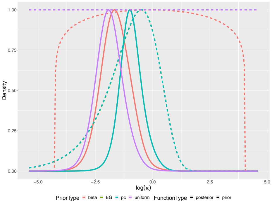
The central claim is that a smooth, invertible parameterization of the correlation length and diffusion matrix of an anisotropic Gaussian field allows construction of penalized complexity priors when the parameters are constant in space. These priors are weakly informative and penalize complexity by pushing the correlation range toward infinity and the anisotropy to zero.
What carries the argument
The smooth invertible parameterization of correlation length and diffusion matrix, used to construct penalized complexity priors.
If this is right
- Bayesian inference for anisotropic Gaussian fields gains a principled weakly informative prior on covariance structure.
- The parameterization supports flexible yet controlled modeling of anisotropy in SPDE-based fields.
- Posteriors are steered away from overly complex short-range or strongly anisotropic fields.
- This construction applies directly when parameters do not vary spatially.
Where Pith is reading between the lines
- The parameterization could be tested for numerical stability in high-dimensional settings with the same prior construction.
- Extensions might explore how the penalization behaves when combined with other likelihood approximations.
- Similar prior ideas could apply to related random field models beyond the SPDE representation.
Load-bearing premise
The correlation length and diffusion matrix parameters are constant in space.
What would settle it
A simulation or dataset where the posterior under this prior fails to push correlation range toward infinity and anisotropy toward zero when the likelihood provides no information on those parameters.
Figures


read the original abstract
Gaussian random fields (GFs) are fundamental tools in spatial modeling and can be represented flexibly and efficiently as solutions to stochastic partial differential equations (SPDEs). The SPDEs depend on specific parameters, which enforce various field behaviors and can be estimated using Bayesian inference. However, even under in-fill asymptotics, the likelihood only provides limited insights into the covariance structure. In response, it is essential to leverage priors to achieve appropriate, meaningful covariance structures in the posterior. This study introduces a smooth, invertible parameterization of the correlation length and diffusion matrix of an anisotropic GF and constructs penalized complexity (PC) priors for the model when the parameters are constant in space. The formulated prior is weakly informative, effectively penalizing complexity by pushing the correlation range toward infinity and the anisotropy to zero.
Editorial analysis
A structured set of objections, weighed in public.
Referee Report
Summary. The manuscript introduces a smooth, invertible parameterization of the correlation length and diffusion matrix for anisotropic Gaussian random fields (GFs) represented via SPDEs. It constructs penalized complexity (PC) priors for these parameters under the restriction that they are spatially constant. The resulting prior is weakly informative and penalizes toward infinite correlation range and zero anisotropy.
Significance. If the parameterization is smooth and invertible and the PC priors are correctly constructed from a valid base model, the work supplies a practical tool for Bayesian spatial modeling with anisotropic fields. The explicit use of the standard PC-prior distance construction (pushing to the base model of infinite range and isotropy) is a strength when the likelihood supplies limited covariance information under in-fill asymptotics.
minor comments (1)
- The abstract states that the parameterization is 'smooth, invertible' and that the prior 'effectively penalizes complexity,' but without the explicit mapping or distance function in the provided description it is not possible to verify that positive-definiteness of the diffusion matrix is preserved for all parameter values.
Simulated Author's Rebuttal
We thank the referee for their summary of the manuscript and for recognizing the practical value of the smooth invertible parameterization together with the PC-prior construction that penalizes toward infinite range and isotropy. We note that the referee report lists no specific major comments.
Circularity Check
No significant circularity; construction is self-contained
full rationale
The paper introduces a smooth invertible reparameterization of correlation length and diffusion matrix for anisotropic Gaussian fields (under the explicit restriction to spatially constant parameters) and then applies the standard penalized complexity prior construction to the resulting parameters. No equation reduces a claimed prediction or uniqueness result to a fitted input by construction, no load-bearing step depends on a self-citation chain whose base result is unverified, and the PC-prior distance penalty toward infinite range and zero anisotropy follows directly from the given base model once the one-to-one mapping is supplied. The derivation therefore consists of an explicit modeling choice rather than an internal reduction.
Axiom & Free-Parameter Ledger
axioms (2)
- domain assumption Gaussian random fields can be represented flexibly as solutions to stochastic partial differential equations
- domain assumption Parameters are constant in space
Reference graph
Works this paper leans on
-
[1]
Adler, R. J., Taylor, J. E., et al. (2007). Random fields and geometry , volume 80. Springer
work page 2007
-
[2]
Banerjee, S., Carlin, B. P., and Gelfand, A. E. (2003). Hierarchical modeling and analysis for spatial data . Chapman and Hall/CRC
work page 2003
-
[3]
Bhatt, S., Weiss, D., Cameron, E., Bisanzio, D., Mappin, B., Dalrymple, U., Battle, K., Moyes, C., Henry, A., Eckhoff, P., et al. (2015). The effect of malaria control on Plasmodium falciparum in Africa between 2000 and 2015. Nature , 526(7572):207--211
work page 2015
-
[4]
Bolin, D., Simas, A. B., and Xiong, Z. (2023). Wasserstein complexity penalization priors: a new class of penalizing complexity priors. arXiv preprint arXiv:2312.04481
-
[5]
Cressie, N. and Wikle, C. K. (2015). Statistics for spatio-temporal data . John Wiley & Sons
work page 2015
-
[6]
Dawid, A. P. and Sebastiani, P. (1999). Coherent dispersion criteria for optimal experimental design. Annals of Statistics , pages 65--81
work page 1999
-
[7]
Dunlop, M. M., Girolami, M. A., Stuart, A. M., and Teckentrup, A. L. (2018). How deep are deep Gaussian processes? Journal of Machine Learning Research , 19(54):1--46
work page 2018
-
[8]
Dunlop, M. M., Iglesias, M. A., and Stuart, A. M. (2017). Hierarchical bayesian level set inversion. Statistics and Computing , 27:1555--1584
work page 2017
-
[9]
Evans, L. C. (2010). Partial differential equations , volume 19. American Mathematical Soc
work page 2010
-
[10]
Fuglstad, G.-A., Lindgren, F., Simpson, D., and Rue, H. (2015). Exploring a new class of non-stationary spatial Gaussian random fields with varying local anisotropy. Statistica Sinica , pages 115--133
work page 2015
-
[11]
Fuglstad, G.-A., Simpson, D., Lindgren, F., and Rue, H. (2019). Constructing priors that penalize the complexity of Gaussian random fields. Journal of the American Statistical Association , 114(525):445--452
work page 2019
-
[12]
Gelbrich, M. (1990). On a formula for the l2 wasserstein metric between measures on euclidean and hilbert spaces. Mathematische Nachrichten , 147(1):185--203
work page 1990
-
[13]
Gel'fand, I. M. and Vilenkin, N. Y. (2014). Generalized functions: Applications of harmonic analysis , volume 4. Academic press
work page 2014
-
[14]
Gneiting, T. and Raftery, A. E. (2007). Strictly proper scoring rules, prediction, and estimation. Journal of the American statistical Association , 102(477):359--378
work page 2007
-
[15]
Grimit, E. P., Gneiting, T., Berrocal, V. J., and Johnson, N. A. (2006). The continuous ranked probability score for circular variables and its application to mesoscale forecast ensemble verification. Quarterly Journal of the Royal Meteorological Society: A journal of the atmospheric sciences, applied meteorology and physical oceanography , 132(621C):2925--2942
work page 2006
-
[16]
Ingebrigtsen, R., Lindgren, F., Steinsland, I., and Martino, S. (2015). Estimation of a non-stationary model for annual precipitation in southern Norway using replicates of the spatial field. Spatial Statistics , 14:338--364
work page 2015
-
[17]
Jaynes, E. T. (2003). Probability theory: The logic of science . Cambridge university press
work page 2003
- [18]
-
[19]
Lindgren, F., Bolin, D., and Rue, H. (2022). The SPDE approach for Gaussian and non- Gaussian fields: 10 years and still running. Spatial Statistics , page 100599
work page 2022
-
[20]
Lindgren, F., Rue, H., and Lindstr \"o m, J. (2011). An explicit link between Gaussian fields and Gaussian Markov random fields: the stochastic partial differential equation approach. Journal of the Royal Statistical Society: Series B (Statistical Methodology) , 73
work page 2011
-
[21]
Lindgren, G. (2012). Stationary stochastic processes: Theory and applications . CRC Press
work page 2012
-
[22]
H., Kim, S., B \"u rkner, P., Huurre, N., Faltejskov \'a , K., Gelman, A., and Vehtari, A
Modr \'a k, M., Moon, A. H., Kim, S., B \"u rkner, P., Huurre, N., Faltejskov \'a , K., Gelman, A., and Vehtari, A. (2023). Simulation-based calibration checking for bayesian computation: The choice of test quantities shapes sensitivity. Bayesian Analysis , 1(1):1--28
work page 2023
-
[23]
Rasmussen, C. E. (2003). Gaussian processes in machine learning. In Summer school on machine learning , pages 63--71. Springer
work page 2003
-
[24]
Roques, L., Allard, D., and Soubeyrand, S. (2022). Spatial statistics and stochastic partial differential equations: A mechanistic viewpoint. Spatial Statistics , 50:100591
work page 2022
-
[25]
Rue, H. and Held, L. (2005). Gaussian Markov random fields: theory and applications . Chapman and Hall/CRC
work page 2005
-
[26]
Sampson, P. D. and Guttorp, P. (1992). Nonparametric estimation of nonstationary spatial covariance structure. Journal of the American Statistical Association , 87(417):108--119
work page 1992
-
[27]
Simpson, D., Lindgren, F., and Rue, H. (2012). Think continuous: Markov ian Gaussian models in spatial statistics. Spatial Statistics , 1:16--29
work page 2012
-
[28]
Simpson, D. P., Rue, H., Martins, T. G., Riebler, A., and S rbye, S. H. (2014). Penalising model component complexity: A principled, practical approach to constructing priors. Statistical Science , 32:1--28
work page 2014
-
[29]
Stein, M. L. (2004). Equivalence of gaussian measures for some nonstationary random fields. Journal of Statistical Planning and Inference , 123(1):1--11
work page 2004
- [30]
-
[31]
Uribe, F., Papaioannou, I., Latz, J., Betz, W., Ullmann, E., and Straub, D. (2021). Bayesian inference with subset simulation in varying dimensions applied to the karhunen–loève expansion. International Journal for Numerical Methods in Engineering , 122(18):5100--5127
work page 2021
- [32]
-
[33]
Wang, J. and Zuo, R. (2021). Spatial modelling of hydrothermal mineralization-related geochemical patterns using INLA + SPDE and local singularity analysis. Computers & Geosciences , 154:104822
work page 2021
-
[34]
Zhang, H. (2004). Inconsistent estimation and asymptotically equal interpolations in model-based geostatistics. Journal of the American Statistical Association , 99(465):250--261
work page 2004
discussion (0)
Sign in with ORCID, Apple, or X to comment. Anyone can read and Pith papers without signing in.