REVIEW 2 major objections 3 minor 1 cited by
New Evidence for a Flux-independent Spectral Index of Sgr A* in the Near-infrared
T0 review · 2 major / 3 minor · reviewed 2026-08-12 · deepseek-v4-flash
Pith's one-line read Seven epochs of ground-based near-infrared imaging show Sgr A*’s spectral index stays constant at −0.50 over a factor of about 40 in brightness, ruling out a purely cutoff-driven synchrotron explanation of its variability.
desk verdict Careful, honest measurement of Sgr A*'s NIR color over the widest range yet; the constant-α conclusion holds for the bright subset and is conditional on assumed confusion colors at the faint end. read the letter →
The pith
A machine-rendered reading of the paper's core claim, the machinery that carries it, and where it could break.
The reading
What carries the argument
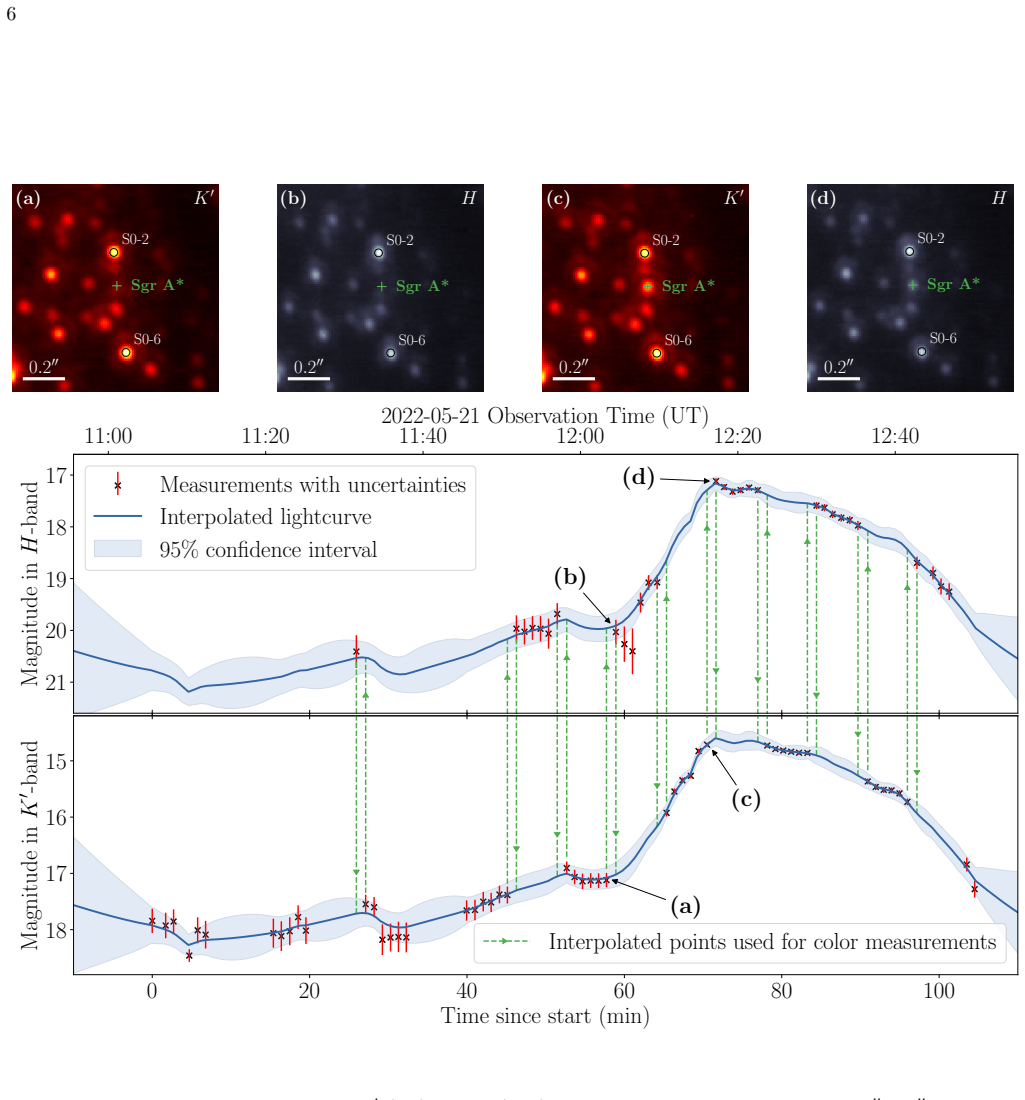
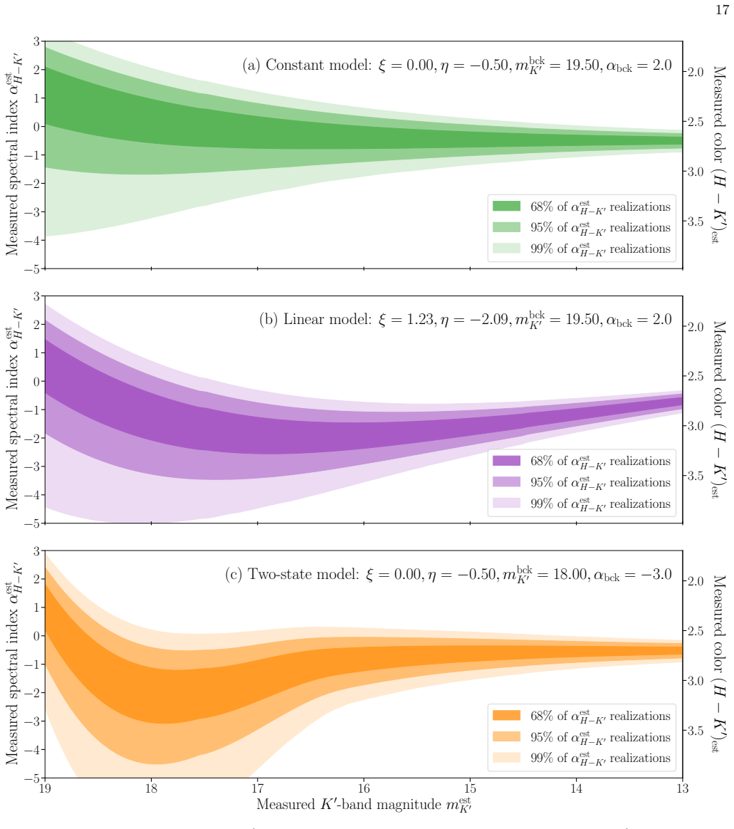
The $H-K^\prime$ spectral index $\alpha$ (with $F_\nu\propto\nu^{\alpha}$) is the central observable, since it tracks the slope of the synchrotron spectrum between 1.6 and 2.2 µm. Two tools carry the analysis: a multi-output Gaussian process (a joint interpolation of the two light curves that lets the correlation between bands be learned rather than fixed) and a four-parameter empirical model (slope $\xi$, intercept $\eta$, background magnitude, background spectral index) that converts an intrinsic spectral index law plus noise and background contamination into predicted measurements. The model’s slope $\xi$ discriminates among scenarios: $\xi=0$ is a constant spectral index, $\xi=1.23$ is the exponential cutoff model, and a bright red background encodes the two-state/quiescent-emission picture. The data prefer $\xi\approx 0$ and constrain the background by marginalizing over it in a Bayesian fit.
What would settle it
Measure the $H$-band magnitudes of S0-38 and S0-104 in epochs when they are not confused with Sgr A*, or with higher-resolution imaging, and recompute the confusion correction with the measured colors. If the true $(H-K^\prime)$ colors deviate substantially from the assumed $0.1\pm0.05$ and $0.0\pm0.1$, the corrected faint spectral indices would shift, and the constant-$\alpha$ conclusion either survives with revised colors or turns into a flux-dependent trend.
Extended reading notes
Core claim
The central claim is that Sgr A*-NIR has a flux-independent spectral index over the largest brightness range yet probed. After removing the flux of two stars confused with the black hole and interpolating between interleaved $H$ and $K^\prime$ frames, the best fit is $\alpha_{H-K^\prime}=-0.50\pm0.08_{\rm stat}\pm0.17_{\rm sys}$, constant from about 1 mJy to about 40 mJy of dereddened 2 µm flux (a factor of roughly 40 in brightness). The linear-slope parameter $\xi$ describing any magnitude dependence is consistent with zero, while the exponential cutoff model, defined by the predicted slope $\xi=1.23$, is excluded at about 5$\sigma$ with the bright subset and about 6$\sigma$ with the extended dataset. The same model places an upper limit of about 0.3 mJy (dereddened 2 µm flux, 95% confidence) on any red, quiescent emission component. The authors conclude that NIR variability is not caused by shifts of the synchrotron cutoff frequency alone and that the variable emission mechanism alters the normalization, not the shape, of the electron energy distribution that produces the NIR radiation.
Load-bearing premise
The load-bearing premise is that the two stars blended with Sgr A* (S0-38 and S0-104) have the assumed intrinsic $H-K^\prime$ colors used to derive their $H$-band magnitudes, since those colors set how much starlight is removed at faint fluxes and therefore determine whether the spectral index stays constant.
Editorial extensions
If this is right
- If the constant spectral index holds, Sgr A*’s near-infrared flares are best explained by a variable number of electrons injected with the same power-law energy distribution ($p\approx 2$), rather than by a moving synchrotron cutoff.
- The exponential cutoff model is excluded as the sole driver of NIR variability, so models must include another mechanism for the flux changes.
- A red quiescent component, if it exists, contributes less than about 0.3 mJy of dereddened 2 µm flux, in tension with earlier two-state model predictions of roughly 0.7–1.1 mJy.
- Earlier reports of dramatic reddening at faint fluxes are likely explained by background subtraction methods or unresolved stellar contamination rather than by the black hole’s intrinsic emission.
- The bright-state spectral index of about $\alpha\approx-0.6$ extends to flux densities about 2.8 times brighter than previously measured, including the 2019 May 13 record flare.
Reading between the lines
- A direct test would be to obtain unconfused $H$-band photometry of S0-38 and S0-104; if their true intrinsic colors are redder or bluer than assumed, the faint-end corrected spectral indices would shift systematically, potentially reviving a flux dependence.
- If the constant index extends to even fainter fluxes with future larger telescopes, the two-state model would need to place its transition below about 0.3 mJy, making the quiescent component nearly invisible.
- Measuring colors across more than two bands (for example $H$, $K^\prime$, and $M$) during the same flares would test whether the spectral energy distribution is a true power law or has curvature that two-band photometry cannot see.
- The same joint-interpolation plus confusion-correction approach could be applied to other crowded-field variable sources, where apparent color–flux trends are often contaminated by unresolved stars.
Signed reviews
Editorial analysis
A structured set of objections, weighed in public.
Referee Report
Summary. The paper analyzes seven epochs (2005, 2019, and 2022) of Keck/NIRC2 imaging of Sgr A* in H and K′ bands, measuring the near-infrared spectral index α (Fν ∝ να) over the largest brightness range studied to date, roughly a factor of 40 in dereddened Ks flux. The analysis includes a star-planting-based correction for two stellar sources confused with Sgr A*, a Multi-Output Gaussian Process interpolation of the interleaved H and K′ lightcurves, and a flexible empirical model with free parameters for the slope ξ of α versus K′ magnitude, the intercept η, and the magnitude and spectral index of any background contribution. The authors find that the data prefer a constant spectral index α = −0.50 ± 0.08_stat ± 0.17_sys over roughly 1–40 mJy, disfavor the exponential-cutoff model of Witzel et al. (2018) at about 5–6σ, and place a 95% upper limit of about 0.3 mJy on redder quiescent emission.
Significance. If the result holds, it is a substantial observational constraint: it extends the flux range over which Sgr A*'s NIR spectral index is constant by roughly a factor of three compared with previous work, and it directly challenges the idea that NIR variability is driven primarily by shifts of the synchrotron cutoff frequency. The paper is unusually careful in several respects: the confusion correction is validated with star-planting simulations, the MOGP interpolation is tested with leave-one-out residuals (Appendix E.3), completeness limits are quantified, and the extinction systematic is separated from statistical error. The Bayesian model comparison is transparent, and the machine-readable table accompanying Figure 4 will be useful to the community. The main weakness identified in this report is a specific robustness gap concerning the assumed intrinsic colors of the confusing stars; the overall methodology is sound.
major comments (2)
- [3.2 / Table 5 / Eq. (2)] The faint-end constancy claim depends on the assumed intrinsic H−K′ colors of the two confusing stars, and this assumption is not stress-tested. S0-38 and S0-104 have no direct H-band measurement; their H magnitudes are set by (H−K′)_int = 0.1 ± 0.05 and 0.0 ± 0.1 (Table 5), and the star-planting correction then subtracts stellar contamination using these values. Equation (2) gives dα/d(H−K′) ≈ −3.5, so a 0.1–0.2 mag error in either star's assumed color, if it propagates into the recovered Sgr A* color, shifts α by roughly 0.35–0.7, several times the quoted statistical error and larger than the quoted 0.17 systematic. Table 4 shows confusion corrections Δα up to 1.88 precisely where the extended dataset adds information. The disappearance of the bluer-when-fainter trend in Figure 3 is therefore partly enforced by subtracting a stellar component whose H-band brightness is an assumption, and cannot by itself validate the correction. I ask the authors to add a robustness test that varies (H−K′)_int for S0-38 and S0-104 by plausible amounts, including a mismatched combination for the spectrally unknown S0-104, re-runs the star-planting/confusion-correction and the Section 5.2 inference, and reports how ξ and η move and whether the constant-α model remains preferred.
- [5.2 / Figure 7 / Table 7] The paper states that the extended dataset rules out the exponential cutoff model at about 6σ and gives a constant α over the full 1–40 mJy range, but the faint end contributes little independent statistical weight and the headline constancy is largely carried by the bright subset. From Figure 7, the ξ posteriors from the bright subset (−0.19+0.22/−0.19) and the extended dataset (0.21+0.17/−0.16) are both within about 1–1.3σ of zero, and Section 5.2 itself notes that most of the constraining power comes from the bright points. This is not a flaw in itself, but it means the claimed full-range constancy is a statement about the absence of a visible faint-end trend in noisier, heavily corrected data. The sensitivity test requested above should therefore be paired with a presentation of the faint-end subsample alone, for example the points with 16.5 < m_K′ < 17.2, showing the fits with ξ = 0 and ξ = 1.23, so that the reader can see how much of the conclusion depends on the faint points as opposed to extrapolation from the bright subset.
minor comments (3)
- [4.1.2 / Eq. (4)] The label 'exponential cutoff model' is defined by fixing ξ = 1.23 while leaving η free; the text should state explicitly that the full Witzel et al. (2018) model also predicts η through Eq. (4), so the 5–6σ exclusion applies to the predicted slope rather than to the complete two-parameter model.
- [5.1 / 5.2] The abstract quotes α = −0.50, while Sections 5.1 and 5.2 and Figure 8 report η = −0.49 ± 0.08; the text should state explicitly that −0.50 is the rounded central value of the extended-dataset posterior to avoid an apparent inconsistency.
- [Appendix G / Eq. (G25)] The derivation of the likelihood in Appendix G is compact because several variables (H_est, F_obs_H,SgrA, F_obs_H,bck) are defined in the flowchart of Figure 5; defining them again in the appendix would make the Jacobian computation in Eq. (G27) easier to verify.
Circularity Check
No significant circularity: the cutoff-slope test is a re-derived, falsifiable prediction and the faint-end color assumption is a stated systematic limitation, not a circular reduction.
full rationale
The central derivation is an empirical fit: ξ, η, m_bck and α_bck are free parameters (Section 4.2, Table 6), and the constant-slope conclusion is drawn from Bayesian evidence/AIC/BIC, not from renaming a fit as a prediction. The one imported quantity that could look load-bearing is the exponential-cutoff slope ξ = 1.23 from Witzel et al. (2018), which shares an author with this paper; however, Section 4.1.2 re-derives that value from wavelength ratios (Eq. 4), and the test uses new Keck data that reject it, so the citation is not being used as unverified support. The faint-end constant-α claim does depend on assumed intrinsic colors for the confusing stars S0-38 and S0-104 (Section 3.2, Table 5), and the paper explicitly flags this as an educated guess in Section 6.3; that is a genuine systematic-uncertainty limitation that could bias the extended dataset, but it is not circular because the colors are set from stellar classification and literature, not from the target spectral index. The bright subset (m_K' < 16.5) independently rules out the cutoff model at about 5σ, so the principal rejection does not rely on the faint-end correction. Overall, no step in the claimed derivation reduces by construction to its own input.
Assumptions & free parameters
free parameters (6)
- ξ (slope of α vs. magnitude) =
−0.19 ± 0.22 (bright); 0.21 ± 0.17 (extended)
- η (spectral index at m0 = 15.8) =
−0.50 ± 0.08 stat, ±0.17 sys
- m_bck^K' (background magnitude in K') =
≥ 20.3 (95%, stellar, extended); ≥ 18.3 (95%, red, extended)
- α_bck (background spectral index) =
Unconstrained; degenerate with η when α_bck ≈ η
- m0_K' (reference magnitude) =
15.8
- Noise law C_band, β_band per night =
e.g., log10 C_K' = −1.56 ± 0.09, β_K' = 0.50 ± 0.03 (Table 3)
assumptions (6)
- domain assumption Additive background plus uncorrelated Gaussian white noise per band (Eq. 7)
- domain assumption Intrinsic spectral index is a linear function of magnitude (Eq. 3)
- domain assumption Color excess derived from S0-2, E(H−K') = 2.07 ± 0.05, applies to Sgr A*
- domain assumption Assumed intrinsic colors of confusing stars: S0-38 (H−K')_int = 0.1 ± 0.05; S0-104 (H−K')_int = 0.0 ± 0.1
- domain assumption MOGP kernel: RBF + exponential + constant + white noise, with 0 ≤ l_exp ≤ 10 min
- domain assumption Cutoff-shift model of Witzel et al. (2018) implies ξ = 1.23
Cite this review
Pith. "Pith review of New Evidence for a Flux-independent Spectral Index of Sgr A* in the Near-infrared." pith.science (2026). https://pith.science/paper/6FDCCB5N
@misc{pith2026241111966,
  author       = {Pith},
  title        = {Pith review of: New Evidence for a Flux-independent Spectral Index of Sgr A* in the Near-infrared},
  year         = {2026},
  howpublished = {\url{https://pith.science/paper/6FDCCB5N}},
  note         = {Machine review of arXiv:2411.11966}
}
abstract
In this work, we measure the spectral index of Sagittarius A* (Sgr A*) between the $H$ (1.6 $\mu$m) and $K^\prime$ (2.2 $\mu$m) broadband filters in the near-infrared (NIR), sampling over a factor $\sim 40$ in brightness, the largest range probed to date by a factor $\sim 3$. Sgr A*-NIR is highly variable, and studying the spectral index $\alpha$ (with $F_\nu \propto \nu^{\alpha}$) is essential to determine the underlying emission mechanism. For example, variations in $\alpha$ with flux may arise from shifts in the synchrotron cutoff frequency, changes in the distribution of electrons, or multiple concurrent emission mechanisms. We investigate potential variations of $\alpha_{H-K^\prime}$ with flux by analyzing 7 epochs (2005 to 2022) of Keck Observatory imaging observations from the Galactic Center Orbits Initiative (GCOI). We remove the flux contribution of known sources confused with Sgr A*-NIR, which can significantly impact color at faint flux levels. We interpolate between the interleaved $H$ and $K^\prime$ observations using Multi-Output Gaussian Processes. We introduce a flexible empirical model to quantify $\alpha$ variations and probe different scenarios. The observations are best fit by an $\alpha_{H-K^\prime} = - 0.50 \pm 0.08 _{\rm stat} \pm 0.17_{\rm sys}$ that is constant from $\sim 1$ mJy to $\sim 40$ mJy (dereddened 2 $\mu$m flux). We find no evidence for a flux-dependence of Sgr A*'s intrinsic spectral index. In particular, we rule out a model explaining NIR variability purely by shifts in the synchrotron cutoff frequency. We also constrain the presence of redder, quiescent emission from the black hole, concluding that the dereddened 2 $\mu$m flux contribution must be $\leq 0.3$ mJy at 95% confidence level.
Figures


Figures from the paper (15 more)




Forward citations
Cited by 1 Pith paper
-
Non-stop Variability of Sgr A* using JWST at 2.1 and 4.8 micron Wavelengths: Evidence for Distinct Populations of Faint and Bright Variable Emission
JWST NIRCam infrared monitoring of Sgr A* finds fully continuous variability on seconds-to-year timescales, a faint/bright two-population flux distribution, and a 3-40 second lag of 4.8 micron behind 2.1 micron emission.
Reference graph
Works this paper leans on
-
[1]
2023, ARA&A, 61, 329, doi: 10.1146/annurev-astro-052920-103508
Aigrain, S., & Foreman-Mackey, D. 2023, ARA&A, 61, 329, doi: 10.1146/annurev-astro-052920-103508
-
[2]
2020, MNRAS, 493, 1404, doi: 10.1093/mnras/staa318 Astropy Collaboration, Robitaille, T
Anantua, R., Ressler, S., & Quataert, E. 2020, MNRAS, 493, 1404, doi: 10.1093/mnras/staa318 Astropy Collaboration, Robitaille, T. P., Tollerud, E. J., et al. 2013, A&A, 558, A33, doi: 10.1051/0004-6361/201322068 Astropy Collaboration, Price-Whelan, A. M., Sip˝ ocz, B. M., et al. 2018, AJ, 156, 123, doi: 10.3847/1538-3881/aabc4f Astropy Collaboration, Pric...
-
[3]
Baganoff, F. K., Bautz, M. W., Brandt, W. N., et al. 2001, Nature, 413, 45, doi: 10.1038/35092510
doi:10.1038/35092510 2001
-
[4]
K., Maeda, Y., Morris, M., et al
Baganoff, F. K., Maeda, Y., Morris, M., et al. 2003, ApJ, 591, 891, doi: 10.1086/375145
doi:10.1086/375145 2003
-
[5]
Balick, B., & Brown, R. L. 1974, ApJ, 194, 265, doi: 10.1086/153242
doi:10.1086/153242 1974
-
[6]
2021, ApJ, 917, 8, doi: 10.3847/1538-4357/abf8ae
Ball, D., ¨Ozel, F., Christian, P., Chan, C.-K., & Psaltis, D. 2021, ApJ, 917, 8, doi: 10.3847/1538-4357/abf8ae
-
[7]
C., Dexter, J., Asada, K., et al
Bower, G. C., Dexter, J., Asada, K., et al. 2019, ApJL, 881, L2, doi: 10.3847/2041-8213/ab3397
-
[8]
2022, ApJ, 931, 7, doi: 10.3847/1538-4357/ac6104
Boyce, H., Haggard, D., Witzel, G., et al. 2022, ApJ, 931, 7, doi: 10.3847/1538-4357/ac6104
Show all 97 references
-
[9]
2011, A&A, 532, A26, doi: 10.1051/0004-6361/201016134
Bremer, M., Witzel, G., Eckart, A., et al. 2011, A&A, 532, A26, doi: 10.1051/0004-6361/201016134
2011 doi
-
[10]
2021, The Journal of Open Source Software, 6, 3001, doi: 10.21105/joss.03001
Buchner, J. 2021, The Journal of Open Source Software, 6, 3001, doi: 10.21105/joss.03001
2021 doi
-
[11]
2018, MNRAS, 478, 5209, doi: 10.1093/mnras/sty1261
Chael, A., Rowan, M., Narayan, R., Johnson, M., & Sironi, L. 2018, MNRAS, 478, 5209, doi: 10.1093/mnras/sty1261
2018 doi
-
[12]
2021, MNRAS, 507, 5281, doi: 10.1093/mnras/stab2466
Chatterjee, K., Markoff, S., Neilsen, J., et al. 2021, MNRAS, 507, 5281, doi: 10.1093/mnras/stab2466
2021 doi
-
[13]
2019, ApJL, 882, L28, doi: 10.3847/2041-8213/ab3c68
Chen, Z., Gallego-Cano, E., Do, T., et al. 2019, ApJL, 882, L28, doi: 10.3847/2041-8213/ab3c68
2019 doi
-
[14]
Connors, R. M. T., Markoff, S., Nowak, M. A., et al. 2017, MNRAS, 466, 4121, doi: 10.1093/mnras/stw3150
2017 doi
-
[15]
2011, MNRAS, 418, 1935, doi: 10.1111/j.1365-2966.2011.19612.x
Contini, M. 2011, MNRAS, 418, 1935, doi: 10.1111/j.1365-2966.2011.19612.x
2011
-
[16]
2018, A&A, 612, A34, doi: 10.1051/0004-6361/201732025
Davelaar, J., Mo´ scibrodzka, M., Bronzwaer, T., & Falcke, H. 2018, A&A, 612, A34, doi: 10.1051/0004-6361/201732025
2018 doi
-
[17]
2020, MNRAS, 497, 4999, doi: 10.1093/mnras/staa2288
Dexter, J., Tchekhovskoy, A., Jim´ enez-Rosales, A., et al. 2020, MNRAS, 497, 4999, doi: 10.1093/mnras/staa2288
2020 doi
-
[18]
2014, MNRAS, 441, 1005, doi: 10.1093/mnras/stu599
Dibi, S., Markoff, S., Belmont, R., et al. 2014, MNRAS, 441, 1005, doi: 10.1093/mnras/stu599
2014 doi
-
[19]
2000, A&AS, 147, 335, doi: 10.1051/aas:2000305
Diolaiti, E., Bendinelli, O., Bonaccini, D., et al. 2000, A&AS, 147, 335, doi: 10.1051/aas:2000305
2000 doi
-
[20]
M., Morris, M
Do, T., Ghez, A. M., Morris, M. R., et al. 2009a, ApJ, 703, 1323, doi: 10.1088/0004-637X/703/2/1323 —. 2009b, ApJ, 691, 1021, doi: 10.1088/0004-637X/691/2/1021
-
[21]
R., Ghez, A
Do, T., Lu, J. R., Ghez, A. M., et al. 2013, ApJ, 764, 154, doi: 10.1088/0004-637X/764/2/154
2013 doi
-
[22]
2019a, Science, 365, 664, doi: 10.1126/science.aav8137
Do, T., Hees, A., Ghez, A., et al. 2019a, Science, 365, 664, doi: 10.1126/science.aav8137
-
[23]
K., et al
Do, T., Witzel, G., Gautam, A. K., et al. 2019b, ApJL, 882, L27, doi: 10.3847/2041-8213/ab38c3
-
[24]
2010, ApJ, 725, 450, doi: 10.1088/0004-637X/725/1/450
Dodds-Eden, K., Sharma, P., Quataert, E., et al. 2010, ApJ, 725, 450, doi: 10.1088/0004-637X/725/1/450
2010 doi
-
[25]
2009, ApJ, 698, 676, doi: 10.1088/0004-637X/698/1/676
Dodds-Eden, K., Porquet, D., Trap, G., et al. 2009, ApJ, 698, 676, doi: 10.1088/0004-637X/698/1/676
2009 doi
-
[26]
K., et al
Dodds-Eden, K., Gillessen, S., Fritz, T. K., et al. 2011, The Astrophysical Journal, 728, 37, doi: 10.1088/0004-637X/728/1/37
2011 doi
-
[27]
2001, ApJ, 558, 309, doi: 10.1086/322439
Ribeiro, D. 2001, ApJ, 558, 309, doi: 10.1086/322439
2001 doi
-
[28]
2006, A&A, 455, 1, doi: 10.1051/0004-6361:20064948
Eckart, A., Sch¨ odel, R., Meyer, L., et al. 2006, A&A, 455, 1, doi: 10.1051/0004-6361:20064948
2006 doi
-
[29]
K., Morris, M., et al
Eckart, A., Baganoff, F. K., Morris, M., et al. 2004, A&A, 427, 1, doi: 10.1051/0004-6361:20040495
2004 doi
-
[30]
K., Morris, M
Eckart, A., Baganoff, F. K., Morris, M. R., et al. 2009, A&A, 500, 935, doi: 10.1051/0004-6361/200811354
2009 doi
-
[31]
N., et al
Eckart, A., Garc ´ ıa-Mar ´ ın, M., Vogel, S. N., et al. 2012, A&A, 537, A52, doi: 10.1051/0004-6361/201117779
2012 doi
- [32]
-
[33]
2005, ApJ, 628, 246, doi: 10.1086/430667 Event Horizon Telescope Collaboration, Akiyama, K.,
Eisenhauer, F., Genzel, R., Alexander, T., et al. 2005, ApJ, 628, 246, doi: 10.1086/430667 Event Horizon Telescope Collaboration, Akiyama, K.,
2005 doi
-
[34]
2022a, ApJL, 930, L16, doi: 10.3847/2041-8213/ac6672 —
Alberdi, A., et al. 2022a, ApJL, 930, L16, doi: 10.3847/2041-8213/ac6672 —. 2022b, ApJL, 930, L12, doi: 10.3847/2041-8213/ac6674
-
[35]
2016, The Journal of Open Source Software, 1, 24, doi: 10.21105/joss.00024
Foreman-Mackey, D. 2016, The Journal of Open Source Software, 1, 24, doi: 10.21105/joss.00024
2016 doi
-
[36]
K., Gillessen, S., Dodds-Eden, K., et al
Fritz, T. K., Gillessen, S., Dodds-Eden, K., et al. 2011, ApJ, 737, 73, doi: 10.1088/0004-637X/737/2/73
2011 doi
-
[37]
K., Do, T., Ghez, A
Gautam, A. K., Do, T., Ghez, A. M., et al. 2019, ApJ, 871, 103, doi: 10.3847/1538-4357/aaf103
2019 doi
-
[38]
K., Do, T., Ghez, A
Gautam, A. K., Do, T., Ghez, A. M., et al. 2024, ApJ, 964, 164, doi: 10.3847/1538-4357/ad26e6
2024 doi
-
[39]
2010, Reviews of Modern Physics, 82, 3121, doi: 10.1103/RevModPhys.82.3121
Genzel, R., Eisenhauer, F., & Gillessen, S. 2010, Reviews of Modern Physics, 82, 3121, doi: 10.1103/RevModPhys.82.3121
2010 doi
-
[40]
2003, Nature, 425, 934, doi: 10.1038/nature02065
Genzel, R., Sch¨ odel, R., Ott, T., et al. 2003, Nature, 425, 934, doi: 10.1038/nature02065
2003 doi
-
[41]
M., Duchˆ ene, G., Matthews, K., et al
Ghez, A. M., Duchˆ ene, G., Matthews, K., et al. 2003, ApJL, 586, L127, doi: 10.1086/374804
2003 doi
-
[42]
M., Wright, S
Ghez, A. M., Wright, S. A., Matthews, K., et al. 2004, ApJL, 601, L159, doi: 10.1086/382024
2004 doi
-
[43]
M., Hornstein, S
Ghez, A. M., Hornstein, S. D., Lu, J. R., et al. 2005, ApJ, 635, 1087, doi: 10.1086/497576
2005 doi
-
[44]
M., Salim, S., Weinberg, N
Ghez, A. M., Salim, S., Weinberg, N. N., et al. 2008, ApJ, 689, 1044, doi: 10.1086/592738
2008 doi
-
[45]
2009a, ApJ, 692, 1075, doi: 10.1088/0004-637X/692/2/1075 —
Gillessen, S., Eisenhauer, F., Trippe, S., et al. 2009a, ApJ, 692, 1075, doi: 10.1088/0004-637X/692/2/1075 —. 2009b, ApJ, 692, 1075, doi: 10.1088/0004-637X/692/2/1075
-
[46]
2006, ApJL, 640, L163, doi: 10.1086/503557
Gillessen, S., Eisenhauer, F., Quataert, E., et al. 2006, ApJL, 640, L163, doi: 10.1086/503557
2006 doi
-
[47]
1997, Geostatistics for Natural Resource
Goovaerts, P. 1997, Geostatistics for Natural Resource
1997
-
[48]
Evaluation, Vol. 42 GPy. since 2012, GPy: A Gaussian process framework in python, http://github.com/SheffieldML/GPy GRA VITY Collaboration, Abuter, R., Amorim, A., et al. 2019, A&A, 625, L10, doi: 10.1051/0004-6361/201935656 —. 2020, A&A, 638, A2, doi: 10.1051/0004-6361/202037...
2012 doi
-
[49]
A., & Dexter, J
Grigorian, A. A., & Dexter, J. 2024, MNRAS, 530, 1563, doi: 10.1093/mnras/stae934 Guti´ errez, E. M., Nemmen, R., & Cafardo, F. 2020, ApJL, 891, L36, doi: 10.3847/2041-8213/ab7998
2024 doi
-
[50]
Ho, L. C. 2008, ARA&A, 46, 475, doi: 10.1146/annurev.astro.45.051806.110546
2008 arXiv
-
[51]
D., Matthews, K., Ghez, A
Hornstein, S. D., Matthews, K., Ghez, A. M., et al. 2007, ApJ, 667, 900, doi: 10.1086/520762
2007 doi
-
[52]
R., Anderson, J., et al
Hosek, Matthew W., J., Lu, J. R., Anderson, J., et al. 2019, ApJ, 870, 44, doi: 10.3847/1538-4357/aaef90 —. 2018, ApJ, 855, 13, doi: 10.3847/1538-4357/aaabbb
2019 doi
-
[53]
E., Stenning, D
Jones, D. E., Stenning, D. C., Ford, E. B., et al. 2022, The Annals of Applied Statistics, 16, 652 , doi: 10.1214/21-AOAS1471
2022 doi
-
[54]
G., & Huijbregts, C
Journel, A. G., & Huijbregts, C. J. 1976, Mining geostatistics, Academic Press
1976
-
[55]
E., et al
Krabbe, A., Iserlohe, C., Larkin, J. E., et al. 2006, ApJL, 642, L145, doi: 10.1086/504587
2006 doi
-
[56]
2004, ApJL, 611, L101, doi: 10.1086/423985
Liu, S., Petrosian, V., & Melia, F. 2004, ApJL, 611, L101, doi: 10.1086/423985
2004 doi
-
[57]
R., Gautam, A
Lu, J. R., Gautam, A. K., Chu, D., Terry, S. K., & Do, T. 2021, Keck-DataReductionPipelines/KAI: v1.0.0 Release of KAI, v1.0.0, Zenodo, doi: 10.5281/zenodo.6677744
2021 doi
-
[58]
Macquart, J.-P., & Bower, G. C. 2006, ApJ, 641, 302, doi: 10.1086/500317
2006 doi
-
[59]
Markoff, S., Falcke, H., Yuan, F., & Biermann, P. L. 2001, A&A, 379, L13, doi: 10.1051/0004-6361:20011346
2001 doi
-
[60]
K., chen, s., et al
Martinez, G., O’Neil, K. K., chen, s., et al. 2022, in American Astronomical Society Meeting Abstracts, Vol. 54, American Astronomical Society Meeting Abstracts, 302.20
2022
-
[61]
C., Morris, M., Walter, F., & Baganoff, F
Mauerhan, J. C., Morris, M., Walter, F., & Baganoff, F. K. 2005, ApJL, 623, L25, doi: 10.1086/429960
2005 doi
-
[62]
2012, Science, 338, 84
Meyer, L., Ghez, A., Sch¨ odel, R., et al. 2012, Science, 338, 84
2012
-
[63]
2021, ApJL, 910, L1, doi: 10.3847/2041-8213/abeb70
Murchikova, L. 2021, ApJL, 910, L1, doi: 10.3847/2041-8213/abeb70
2021 doi
-
[64]
1995, Nature, 374, 623, doi: 10.1038/374623a0
Narayan, R., Yi, I., & Mahadevan, R. 1995, Nature, 374, 623, doi: 10.1038/374623a0
1995 doi
-
[65]
2008, ApJ, 680, 1174, doi: 10.1086/587791
Nishiyama, S., Nagata, T., Tamura, M., et al. 2008, ApJ, 680, 1174, doi: 10.1086/587791
2008 doi
-
[66]
2006, ApJ, 638, 839, doi: 10.1086/499038
Nishiyama, S., Nagata, T., Kusakabe, N., et al. 2006, ApJ, 638, 839, doi: 10.1086/499038
2006 doi
-
[67]
2019, A&A, 630, L3, doi: 10.1051/0004-6361/201936322
Nogueras-Lara, F., Sch¨ odel, R., Najarro, F., et al. 2019, A&A, 630, L3, doi: 10.1051/0004-6361/201936322
2019 doi
-
[68]
2020, A&A, 641, A141, doi: 10.1051/0004-6361/202038606
Nogueras-Lara, F., Sch¨ odel, R., Neumayer, N., et al. 2020, A&A, 641, A141, doi: 10.1051/0004-6361/202038606
2020 doi
-
[69]
T., Dong, H., et al
Nogueras-Lara, F., Gallego-Calvente, A. T., Dong, H., et al. 2018, A&A, 610, A83, doi: 10.1051/0004-6361/201732002
2018 doi
-
[70]
2006, ApJ, 643, 1011, doi: 10.1086/503273
Paumard, T., Genzel, R., Martins, F., et al. 2006, ApJ, 643, 1011, doi: 10.1086/503273
2006 doi
-
[71]
2017, MNRAS, 468, 2447, doi: 10.1093/mnras/stx596
Ponti, G., George, E., Scaringi, S., et al. 2017, MNRAS, 468, 2447, doi: 10.1093/mnras/stx596
2017 doi
-
[72]
2008, A&A, 488, 549–557, doi: 10.1051/0004-6361:200809986
Porquet, D., Grosso, N., Predehl, P., et al. 2008, A&A, 488, 549–557, doi: 10.1051/0004-6361:200809986
2008 doi
-
[73]
2021, Monthly Notices of the Royal Astronomical Society, 502, 2023 42
Porth, O., Mizuno, Y., Younsi, Z., & Fromm, C. 2021, Monthly Notices of the Royal Astronomical Society, 502, 2023 42
2021
-
[74]
2015, MNRAS, 452, 2269, doi: 10.1093/mnras/stv1428
Roberts, S. 2015, MNRAS, 452, 2269, doi: 10.1093/mnras/stv1428
2015 doi
-
[75]
E., & Williams, C
Rasmussen, C. E., & Williams, C. K. I. 2005, Gaussian Processes for Machine Learning (The MIT Press), doi: 10.7551/mitpress/3206.001.0001
2005 doi
-
[76]
M., White, C
Ressler, S. M., White, C. J., & Quataert, E. 2023, MNRAS, 521, 4277, doi: 10.1093/mnras/stad837
2023 doi
-
[77]
Ripperda, B., Bacchini, F., & Philippov, A. A. 2020, ApJ, 900, 100, doi: 10.3847/1538-4357/ababab
2020 doi
-
[78]
R., Ghez, A., et al
Sakai, S., Lu, J. R., Ghez, A., et al. 2019, ApJ, 873, 65, doi: 10.3847/1538-4357/ab0361 Sch¨ odel, R., Najarro, F., Muzic, K., & Eckart, A. 2010, A&A, 511, A18, doi: 10.1051/0004-6361/200913183 Sch¨ odel, R., Ott, T., Genzel, R., et al. 2003, ApJ, 596, 1015, doi: 10.1086/378122
2019 doi
-
[79]
2017, A&A, 601, A80, doi: 10.1051/0004-6361/201628530
Subroweit, M., Garc ´ ıa-Mar ´ ın, M., Eckart, A., et al. 2017, A&A, 601, A80, doi: 10.1051/0004-6361/201628530
2017 doi
-
[80]
W., Seeger, M., & Jordan, M
Teh, Y. W., Seeger, M., & Jordan, M. I. 2005, in International Workshop on Artificial Intelligence and
2005
- [81]
- [82]
-
[83]
2020, Applied Sciences, 10, doi: 10.3390/app10196765
Torres-Valencia, C., Orozco, A., C´ ardenas-Pe˜ na, D., ´Alvarez Meza, A., & ´Alvarez, M. 2020, Applied Sciences, 10, doi: 10.3390/app10196765
2020 doi
-
[84]
2011, A&A, 528, A140, doi: 10.1051/0004-6361/201015157
Trap, G., Goldwurm, A., Dodds-Eden, K., et al. 2011, A&A, 528, A140, doi: 10.1051/0004-6361/201015157
2011 doi
-
[85]
2007, Monthly Notices of the Royal Astronomical Society, 375, 764 van Dam, M
Trippe, S., Paumard, T., Ott, T., et al. 2007, Monthly Notices of the Royal Astronomical Society, 375, 764 van Dam, M. A., Mignant, D. L., & Macintosh, B. A. 2004, Appl. Opt., 43, 5458, doi: 10.1364/AO.43.005458
2007 doi
-
[86]
C., Do, T., Witzel, G., et al
Weldon, G. C., Do, T., Witzel, G., et al. 2023, ApJL, 954, L33, doi: 10.3847/2041-8213/acf2f2
2023 doi
-
[87]
2008, in Advances in Neural Information Processing Systems, ed
Williams, C., Klanke, S., Vijayakumar, S., & Chai, K. 2008, in Advances in Neural Information Processing Systems, ed. D. Koller, D. Schuurmans, Y. Bengio, & L. Bottou, Vol. 21 (Curran Associates, Inc.). https://proceedings.neurips.cc/paper files/paper/2008/ file/15d4e891d78497...
2008
-
[88]
2014, in The Galactic Center: Feeding and Feedback in a Normal Galactic Nucleus, ed
Witzel, G., Morris, M., Ghez, A., et al. 2014, in The Galactic Center: Feeding and Feedback in a Normal Galactic Nucleus, ed. L. O. Sjouwerman, C. C. Lang, & J. Ott, Vol. 303, 274–282, doi: 10.1017/S1743921314000738
2014 doi
-
[89]
R., Ghez, A
Witzel, G., Lu, J. R., Ghez, A. M., et al. 2016, in Society of Photo-Optical Instrumentation Engineers (SPIE) Conference Series, Vol. 9909, Adaptive Optics Systems V, ed. E. Marchetti, L. M. Close, & J.-P. V´ eran, 99091O, doi: 10.1117/12.2233872
2016 doi
-
[90]
2018, ApJ, 863, 15, doi: 10.3847/1538-4357/aace62
Witzel, G., Martinez, G., Hora, J., et al. 2018, ApJ, 863, 15, doi: 10.3847/1538-4357/aace62
2018 doi
-
[91]
P., et al
Witzel, G., Martinez, G., Willner, S. P., et al. 2021, ApJ, 917, 73, doi: 10.3847/1538-4357/ac0891
2021 doi
-
[92]
L., Le Mignant, D., Bouchez, A
Wizinowich, P. L., Le Mignant, D., Bouchez, A. H., et al. 2006, PASP, 118, 297, doi: 10.1086/499290
2006 doi
-
[93]
R., Ghez, A
Yelda, S., Lu, J. R., Ghez, A. M., et al. 2010, ApJ, 725, 331, doi: 10.1088/0004-637X/725/1/331
2010 doi
-
[94]
2014, ARA&A, 52, 529, doi: 10.1146/annurev-astro-082812-141003
Yuan, F., & Narayan, R. 2014, ARA&A, 52, 529, doi: 10.1146/annurev-astro-082812-141003
2014 doi
-
[95]
2003, ApJ, 598, 301, doi: 10.1086/378716
Yuan, F., Quataert, E., & Narayan, R. 2003, ApJ, 598, 301, doi: 10.1086/378716
2003 doi
-
[96]
2004, ApJ, 606, 894, doi: 10.1086/383117
Yuan, F., Quataert, E., & Narayan, R. 2004, ApJ, 606, 894, doi: 10.1086/383117
2004 doi
-
[97]
2012, AJ, 144, 1, doi: 10.1088/0004-6256/144/1/1 ´Alvarez, M
Yusef-Zadeh, F., Wardle, M., Dodds-Eden, K., et al. 2012, AJ, 144, 1, doi: 10.1088/0004-6256/144/1/1 ´Alvarez, M. A., & Lawrence, N. D. 2011, The Journal of Machine Learning Research, 12, 1459 ´Alvarez, M. A., Rosasco, L., & Lawrence, N. D. 2012, Foundations and Trends in Mach...
2012 doi
Reviewed August 12, 2026 · model on record in the stance chip above.
Discussion (0). Continue with ORCID to comment.