REVIEW 2 major objections 4 minor 31 references
Nonlinear orbital stability of stationary shock profiles for the Lax-Wendroff scheme
T0 review · 2 major / 4 minor · reviewed 2026-08-12 · deepseek-v4-flash
Pith's one-line read The paper proves that spectrally stable stationary shock profiles of the Lax-Wendroff scheme are nonlinearly orbitally stable: small perturbations converge to the shock profile carrying the perturbation's mass.
desk verdict Solid linear theory, overreaching nonlinear theorem: Theorem 2.5's ℓ∞ decay needs β≥1/3, not the stated β+σ≥5/12 range. read the letter →
The pith
A machine-rendered reading of the paper's core claim, the machinery that carries it, and where it could break.
The reading
What carries the argument
The load-bearing object is the Lopatinskii determinant $\Delta(z)$, an explicitly computable holomorphic function that acts as a characteristic polynomial for the linearized scheme; it is assembled from the roots of the dispersion relations on the two sides of the shock. A simple zero at $z=1$ locates the neutral eigenvalue coming from the one-parameter family of profiles, and non-vanishing of $\Delta$ on the closed exterior of the spectral ellipse of (2.13) is exactly spectral stability. From $\Delta$ the paper builds the spatial Green's function, isolates its pole at $z=1$ with residue $H_j$ (the eigenvector), applies an inverse Laplace transform, and obtains the temporal Green's function whose leading term is the activation function $A(x,y)$ — a primitive of the free Green's function of the Lax-Wendroff transport equation — controlling how the mass of the initial condition accumulates along the eigenvector. The remainder terms are bounded by the functions $M_\ell,M_r,K_\ell,K_r$ encoding the oscillatory-diffusive profile of the dispersive scheme. Polynomial weights $\ell^p_\gamma$ enter because the free Green's function has the known sharp $n^{1/8}$ growth in $\ell^1$, so the weights compensate the weak instability and make the nonlinear bootstrap close.
What would settle it
Take the non-convex construction of Section 3.4 — a shock with $u_\ell=1$, $u_r=-1$, flux values $f(\pm1)=1$, and parameters $(\alpha_\ell,\alpha_r)=(1/3,-2/3)$ with a small oscillation tuning $\alpha_m\approx 8.79$ — for which the paper's formulas give $\Delta(2)=0$: running the scheme with a small perturbation should show growth rather than convergence, confirming that Assumption 1 is genuine. Alternatively, for any flux where sampling $\Delta$ on the spectral curve shows no extra zeros, the theory predicts the exact algebraic decay rates $n^{-\sigma}$ and $n^{-\sigma-11/24}$; a numerical run deviating from these exponents would break the central claim.
Extended reading notes
Core claim
Under the Rankine-Hugoniot relation, the Lax entropy inequalities $f'(u_r)<0<f'(u_\ell)$, the CFL restriction $\max(\alpha_\ell,|\alpha_r|)<1$, and Assumption 1 on the zeros of the Lopatinskii determinant, the paper proves that the family of stationary discrete shock profiles $\{v^\theta\}$ is nonlinearly orbitally stable. Concretely (Theorem 2.5), for any perturbation $h$ of the reference shock $u$ with $\|h\|_{\ell^1_\gamma}$ small enough, the numerical solution $u^n$ is well defined and satisfies $\|p_n\|_{\ell^1_\beta}\le C_0(1+n)^{-\sigma}\|h\|_{\ell^1_\gamma}$ and $\|p_n\|_{\ell^\infty_\beta}\le C_0(1+n)^{-\sigma-11/24}\|h\|_{\ell^1_\gamma}$ for $p_n=u^n-v^\theta$, with $\theta=\sum_j h_j$ and $\gamma=\sigma+\beta+1/8$. The paper also proves that every convex or concave flux satisfies Assumption 1, so for such fluxes — Burgers's equation included — every Lax entropy shock is orbitally stable; and it exhibits non-convex fluxes for which Assumption 1 fails, showing the assumption is not vacuous.
Load-bearing premise
The result rests on the premise, not proved in full generality, that the linearized scheme has no eigenvalue outside the unit disk except the neutral eigenvalue $1$ (a simple zero of the Lopatinskii determinant) — a condition the paper verifies only for convex or concave fluxes and shows can fail for non-convex ones.
Editorial extensions
If this is right
- For any convex or concave flux satisfying the Lax entropy inequalities and the CFL condition, stationary shock profiles of the Lax-Wendroff scheme are nonlinearly orbitally stable; the Burgers-equation shocks used in the numerical experiments are covered.
- Conservation forces the selection of the limit: the asymptotic profile is the one whose excess mass equals the total mass of the initial perturbation, so stability holds for the whole one-parameter family $\{v^\theta\}$, not for a single profile.
- Decay is purely algebraic, at rates $n^{-\sigma}$ in $\ell^1_\beta$ and $n^{-\sigma-11/24}$ in $\ell^\infty_\beta$, because the eigenvalue $1$ is embedded in the continuous spectrum and there is no spectral gap; exponential convergence cannot be expected in this setting.
- The zero-weight case of the linear theory recovers the sharp $n^{1/8}$ growth of the Lax-Wendroff scheme in $\ell^1$, confirming in the shock context that uniform $\ell^1$ stability is impossible and that weighted spaces are the natural framework.
- The constraint $\beta+\sigma\ge 5/12$ with $0\le\sigma<\beta+1/8$ quantifies exactly which polynomial weights allow the bootstrap argument to close.
Reading between the lines
- The authors leave a direct test implicit: because $\Delta$ is explicitly computable, Assumption 1 can be checked numerically for any proposed flux by sampling the determinant on the spectral curve; the non-convex examples of Section 3.4 show where such a check would find failures.
- The activation-function machinery is likely the template for stability analysis of other higher-order dispersive schemes: the embedded neutral eigenvalue, the mass-accumulation function, and polynomial weights compensating dispersive growth should transfer, with exponents changing but the mechanism persisting.
- One may read the sharp $n^{1/8}$ growth as intrinsic to second-order accuracy, suggesting a general principle that no uniform-in-time $\ell^1$ stability theory can exist for such schemes, so weighted spaces are the natural habitat of their stability statements.
- Appendix A's sharp bounds on the activation function supply the key estimate for a local limit theorem for dispersive finite-difference approximations of transport, a connection the paper flags as work in progress rather than develops.
Editorial analysis
A structured set of objections, weighed in public.
Referee Report
Summary. The paper analyzes the spectral, linear, and nonlinear stability of the piecewise constant stationary shock profile (2.7) for the Lax-Wendroff scheme (2.5)-(2.6) for scalar conservation laws. It introduces a Lopatinskii determinant (3.3) whose zero set locates the spectrum of the linearized operator L, proves for convex or concave fluxes that the only zero in the closed exterior region is the simple eigenvalue 1 (Lemma 3.2), and formulates Assumption 1 under which L has no other spectrum in the closed exterior (Theorem 2.3). The central technical content is a detailed construction of the spatial Green's function (Proposition 3.1), a decomposition of the temporal Green's function into an activation-function contribution and remainder terms governed by free constant-coefficient Green's functions (Theorem 4.1), and resulting linear decay estimates in polynomially weighted spaces (Theorem 4.3, (4.37a)-(4.38c)). A bootstrap argument in Chapter 5 uses these estimates to prove orbital stability of the family of stationary shock profiles (Theorem 2.5) for small perturbations, with rates ||p^n||_{ℓ1_β} ≤ C0(1+n)^{-σ}||h||_{ℓ1_γ} and ||p^n||_{ℓ∞_β} ≤ C0(1+n)^{-σ-11/24}||h||_{ℓ1_γ}.
Significance. If the parameter-range issue identified below is corrected, the paper would be a significant contribution to the stability theory of high-order numerical schemes for hyperbolic conservation laws. The explicit Lopatinskii determinant analysis for convex and concave fluxes, the fully written spatial Green's function formulas, and the sharp oscillatory integral estimates in Appendix A are concrete and checkable contributions, and the paper is honest about the failure of uniform ℓ1 estimates and about the conditional nature of Assumption 1. The conditional nonlinear stability theorem is a substantial extension of prior parabolic-type results to a dispersive setting. However, the main theorem as stated is not proven on its full parameter range because the proof uses linear and nonlinear semigroup estimates with exponents that are valid only under hidden restrictions on β. This is a load-bearing flaw that requires a corrected statement or a modified proof.
major comments (2)
- [§5.2.2, Eq. (4.37b)] The ℓ∞_β bound for the linear term L^{n+1}p0 in the induction step is claimed as C_L(β,γ)(2+n)^{-σ-11/24}||p0||_{ℓ1_γ}. Substituting γ1=β and γ2=γ=σ+β+1/8 into Theorem 4.3(4.37b) gives the exponent γ2−γ1+min(1/3,γ1) = σ+1/8+min(1/3,β), which equals σ+11/24 only when β≥1/3. For β<1/3 the exponent is σ+β+1/8, which is strictly smaller than σ+11/24, so the claimed inequality is not a consequence of (4.37b). The theorem statement allows β<1/3, for example β=0.3 and σ=0.125 satisfy β+σ≥5/12 and σ<β+1/8, but the decay bound used in the proof fails for such parameters. The proof therefore establishes Theorem 2.5 only on the restricted range β≥1/3, or with a slower ℓ∞ rate, and the statement must be corrected accordingly.
- [§5.2.2, Eqs. (4.38b)-(4.38c)] In bounding the two nonlinear sums in the ℓ∞_β estimate, the proof replaces the factors min(1/4,β) and min(1/8,β−1/8) in (4.38b) and (4.38c) by 1/4 and 1/8, respectively, using the denominators (1+n−m)^{β+7/12} and (1+n−m)^{β+1/8}. These replacements require β≥1/4; for β<1/4 the correct exponents are 2β+1/3 and β+min(1/8,β−1/8), which are smaller than the ones used. This is a second hidden restriction in the stated parameter range. The more restrictive condition β≥1/3 imposed by the linear term subsumes it, but if the authors choose instead to weaken the ℓ∞ rate, the nonlinear part of the bootstrap would still require β≥1/4.
minor comments (4)
- [Various] The manuscript contains several typographical errors, including 'Thank's' on p. 55, 'avoir' on p. 5, 'perurbation' on p. 16, and 'encompasses' on p. 20; these should be corrected in a revision.
- [§3.4] The two instability examples are convincing in outline, but the phrase "can be achieved by tuning small amplitude oscillations near the origin" is informal; a precise construction of the flux f with the stated derivative values would make the examples fully reproducible.
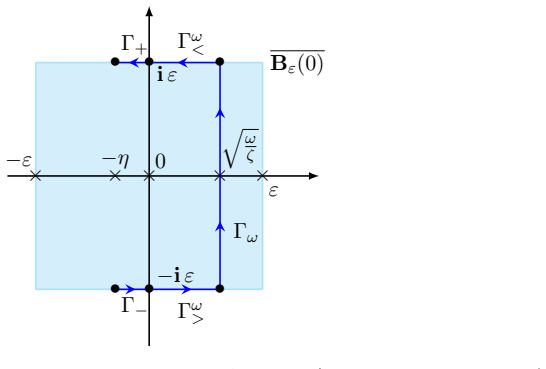
- [§3.2, (3.21)] The notation for B_ε(0) and B_ε(0) in the definition of the region Z_{ε*,η*} is not visually distinct enough in print; the reader must carefully track which of the round or square balls is intended, so a clearer notation or an explicit reminder at each occurrence would help.
- [§5.1] The constants C1 and C2 in §5.1 are defined by long displays that are hard to parse; splitting them into separate displayed summands and explicitly recording the hypothesis on β used for each application of Lemma 5.3 would improve readability.
Circularity Check
No circular derivation: spectral stability is a hypothesis, and the Green's function and decay estimates are derived, not fitted; self-citations to [9] and [7] are prior published analyses, not load-bearing reductions.
full rationale
The paper's central chain is conditional: Assumption 1 (Section 3.2) posits that the Lopatinskii determinant Delta has a simple zero at 1 and no other zero in U\{1}; this is exactly spectral stability, not the target nonlinear result. The Green's function construction (Proposition 3.1), its meromorphic decomposition (Proposition 3.3) and the linear decay estimates (Theorems 4.1-4.3) are proved in the paper from the resolvent problem and the dispersion relations, with Appendix A supplying the free Green's function bounds. The nonlinear bootstrap (Chapter 5) applies Theorem 4.3 to the Duhamel formula; it does not import the conclusion. Citations to [9] (by one author) and [7] provide the free Green's function estimates and the algebraic nonlinear estimate Lemmas 5.1-5.2; these are published proofs with stated hypotheses that do not include Theorem 2.5, so by the review rules they are independent support rather than self-citation circularity. Assumption 1 is explicitly flagged as open to verification ('Our hope is that Assumption 1 can be easily verified (or proved not to hold) in specific situations'), which is an honest limitation, not a concealed input. The skeptical exponent mismatch in §5.2.2 (for beta<1/3, Theorem 4.3(4.37b) yields n^{-sigma-beta-1/8}, not n^{-sigma-11/24}) is a correctness gap on the stated parameter range, not a circularity, and does not change the score.
Assumptions & free parameters
free parameters (2)
- gamma := sigma + beta + 1/8 =
sigma + beta + 1/8
- nu2 := 7/12 + (sigma - 7/12)_+ =
7/12 + (sigma - 7/12)_+
assumptions (7)
- standard math Levy-Wiener theorem and spectral theory of convolution operators on ell-q
- standard math Inverse Laplace transform representation of the semigroup (Equation 4.2)
- domain assumption Rankine-Hugoniot relation (2.3) and Lax entropy inequalities (2.4)
- domain assumption CFL condition max(alpha_l, |alpha_r|) < 1 (2.12)
- domain assumption Assumption 1: Delta has a simple zero at 1 and no other zero in the closed exterior of the spectral curve
- domain assumption Existence of the one-parameter family v_theta of shock profiles with exponential localization (Theorem 2.1)
- domain assumption Sharp bounds for the free Green's functions of L_l and L_r (Theorems A.2, A.3, Corollary A.1)
invented entities (2)
-
Activation functions A_l and A_r (Equation 4.5) and the 'activation function' terminology
-
The Lopatinskii determinant Delta (Equation 3.3)
Cite this review
Pith. "Pith review of Nonlinear orbital stability of stationary shock profiles for the Lax-Wendroff scheme." pith.science (2026). https://pith.science/paper/J2W5DZTV
@misc{pith2026241113094,
  author       = {Pith},
  title        = {Pith review of: Nonlinear orbital stability of stationary shock profiles for the Lax-Wendroff scheme},
  year         = {2026},
  howpublished = {\url{https://pith.science/paper/J2W5DZTV}},
  note         = {Machine review of arXiv:2411.13094}
}
abstract
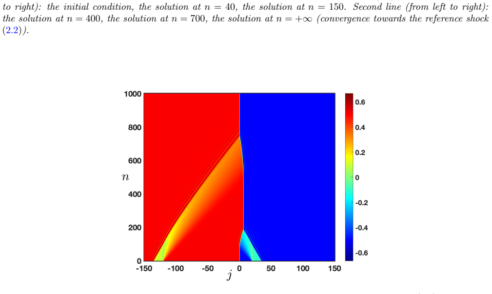
In this article we study the spectral, linear and nonlinear stability of stationary shock profile solutions to the Lax-Wendroff scheme for hyperbolic conservation laws. We first clarify the spectral stability of such solutions depending on the convexity of the flux for the underlying conservation law. The main contribution of this article is a detailed study of the so-called Green's function for the linearized numerical scheme. As evidenced on numerical simulations, the Green's function exhibits a highly oscillating behavior ahead of the leading wave before this wave reaches the shock location. One of our main results gives a quantitative description of this behavior. Because of the existence of a one-parameter family of stationary shock profiles, the linearized numerical scheme admits the eigenvalue 1 that is embedded in its continuous spectrum, which gives rise to several contributions in the Green's function. Our detailed analysis of the Green's function describes these contributions by means of a so-called activation function. For large times, the activation function describes how the mass of the initial condition accumulates along the eigenvector associated with the eigenvalue 1 of the linearized numerical scheme. We can then obtain sharp decay estimates for the linearized numerical scheme in polynomially weighted spaces, which in turn yield a nonlinear orbital stability result for spectrally stable stationary shock profiles. This nonlinear result is obtained despite the lack of uniform ${\ell}$ 1 estimates for the Green's function of the linearized numerical scheme, the lack of such estimates being linked with the dispersive nature of the numerical scheme. This dispersive feature is in sharp contrast with previous results on the orbital stability of traveling waves or discrete shock profiles for parabolic perturbations of conservation laws.
Figures


Figures from the paper (11 more)




Reference graph
Works this paper leans on
- [9]
-
[7]
L. Coeuret. Nonlinear orbital stability of stationary discrete shock profiles for scalar conservation laws. Preprint, arXiv:2409.18930 [math.AP] (2024), 2024
work page Pith review arXiv 2024
-
[1]
S. Benzoni-Gavage, P. Huot, and F. Rousset. Nonlinear stability of semidiscrete shock waves. SIAM J. Math. Anal. , 35(3):639–707, 2003
work page 2003
-
[2]
S. Benzoni-Gavage and D. Serre. Multi-dimensional hyperbolic partial differential equations. First- order systems and applications . Oxford Math. Monogr. Oxford: Oxford University Press, 2007
work page 2007
-
[3]
D. Bouche and W. Weens. Analyse quantitative des sch´ emas num´ eriques pour les ´ equations aux d´ eriv´ ees partielles. Les Ulis: EDP Sciences, 2024
work page 2024
- [4]
-
[5]
M. Bultelle, M. Grassin, and D. Serre. Unstable Godunov discrete profiles for steady shock waves. SIAM J. Numer. Anal. , 35(6):2272–2297, 1998
work page 1998
-
[6]
L. Coeuret. Linear stability of discrete shock profiles for systems of conservation laws. Preprint, arXiv:2311.02507 [math.NA] (2023), 2023
work page Pith review arXiv 2023
Show all 31 references
-
[8]
J. B. Conway. A course in functional analysis . Graduate Texts in Mathematics. Springer-Verlag, 1990
1990
-
[10]
Coulombel and G
J.-F. Coulombel and G. Faye. Generalized Gaussian bounds for discrete convolution powers. Rev. Mat. Iberoam., 38(5):1553–1604, 2022
2022
-
[11]
Coulombel and G
J.-F. Coulombel and G. Faye. The local limit theorem for complex valued sequences: the parabolic case. C. R., Math., Acad. Sci. Paris , 2024
2024
-
[12]
C. M. Dafermos. Hyperbolic conservation laws in continuum physics , volume 325 of Grundlehren der mathematischen Wissenschaften . Springer-Verlag, 2016
2016
-
[13]
Estep, M
D. Estep, M. Loss, and J. Rauch. Boundedness of dispersive difference schemes. Math. Comp. , 55(191):55–87, 1990. 135
1990
-
[14]
Godillon
P. Godillon. Green’s function pointwise estimates for the modified Lax-Friedrichs scheme. M2AN Math. Model. Numer. Anal. , 37(1):1–39, 2003
2003
-
[15]
Harten, J
A. Harten, J. M. Hyman, and P. D. Lax. On finite-difference approximations and entropy conditions for shocks. Comm. Pure Appl. Math. , 29(3):297–322, 1976. With an appendix by B. Keyfitz
1976
-
[16]
G. W. Hedstrom. The near-stability of the Lax-Wendroff method. Numer. Math. , 7:73–77, 1965
1965
-
[17]
G. W. Hedstrom. Norms of powers of absolutely convergent Fourier series. Michigan Math. J. , 13:393–416, 1966
1966
-
[18]
Jennings
G. Jennings. Discrete shocks. Commun. Pure Appl. Math. , 27:25–37, 1974
1974
-
[19]
Kr¨ oner.Numerical schemes for conservation laws
D. Kr¨ oner.Numerical schemes for conservation laws . Wiley-Teubner Series Advances in Numerical Mathematics. John Wiley & Sons, Ltd., Chichester; B. G. Teubner, Stuttgart, 1997
1997
-
[20]
Lax and B
P. Lax and B. Wendroff. Systems of conservation laws. Comm. Pure Appl. Math. , 13:217–237, 1960
1960
-
[21]
R. J. LeVeque. Finite volume methods for hyperbolic problems . Cambridge Texts in Applied Mathe- matics. Cambridge University Press, Cambridge, 2002
2002
-
[22]
D. J. Newman. A simple proof of Wiener’s 1 /f theorem. Proc. Amer. Math. Soc., 48:264–265, 1975
1975
-
[23]
V. V. Petrov. Sums of independent random variables. Translated from the Russian by A. A. Brown , volume 82 of Ergeb. Math. Grenzgeb. Springer-Verlag, Berlin, 1975
1975
-
[24]
Randles and L
E. Randles and L. Saloff-Coste. On the convolution powers of complex functions on Z. J. Fourier Anal. Appl., 21(4):754–798, 2015
2015
-
[25]
Randles and L
E. Randles and L. Saloff-Coste. Convolution powers of complex functions on Zd. Rev. Mat. Iberoam., 33(3):1045–1121, 2017
2017
-
[26]
D. Serre. Systems of conservation laws. 1 . Cambridge University Press, 1999
1999
-
[27]
D. Serre. Discrete shock profiles: existence and stability. In Hyperbolic systems of balance laws , volume 1911 of Lecture Notes in Math. , pages 79–158. Springer, 2007
1911
-
[28]
Y. S. Smyrlis. Existence and stability of stationary profiles of the L W scheme. Comm. Pure Appl. Math., 43(4):509–545, 1990
1990
-
[29]
Thom´ ee
V. Thom´ ee. Stability of difference schemes in the maximum-norm. J. Differential Equations , 1:273– 292, 1965
1965
-
[30]
L. N. Trefethen and M. Embree. Spectra and pseudospectra. Princeton University Press, 2005. The behavior of nonnormal matrices and operators
2005
-
[31]
J. X. Xin. Multidimensional stability of traveling waves in a bistable reaction-diffusion equation. I. Commun. Partial Differ. Equations , 17(11-12):1889–1899, 1992. 136
1992
Reviewed August 12, 2026 · model on record in the stance chip above.
Discussion (0). Continue with ORCID to comment.