REVIEW 2 major objections 5 minor 43 references
Solver-in-the-loop approach to closure of shell models of turbulence
T0 review · 2 major / 5 minor · reviewed 2026-08-12 · deepseek-v4-flash
Pith's one-line read A neural closure trained inside the solver reproduces the highest-order statistics of shell-model turbulence.
desk verdict Solid demonstration that unrolled training beats a priori for shell-model closure, but the physical 'ideal time' claim is post hoc and the locality assumption is under-tested. read the letter →
The pith
A machine-rendered reading of the paper's core claim, the machinery that carries it, and where it could break.
The reading
What carries the argument
The load-bearing mechanism is the differentiable solver. The reduced Sabra system is written in an automatic-differentiation framework; at each step the MLP outputs the two missing shells $\tilde{u}_{N_c+1}, \tilde{u}_{N_c+2}$ from the three preceding shells, and the Runge-Kutta integrator advances the resolved shells for $m_{\text{steps}}$ times. Backpropagation then flows through the solver to update the MLP. The loss is the mean squared error between the LES-NN and ground-truth velocity fields over the six shells below the cutoff, so the network is trained under equation-consistent input distributions rather than static pairs.
What would settle it
A systematic convergence study on the number of input shells: if accuracy on the flatness of order 10 or on the flux pdf at the cutoff improves markedly when the input window is widened from three to, e.g., six shells, the locality assumption underlying the closure would be false. Alternatively, training the same method at a different cutoff (e.g., $N_c=20$) and checking whether the optimal unrolling time still scales with the new cutoff's eddy turnover time would test the paper's physical rule for $m_{\text{steps}}$.
Extended reading notes
Core claim
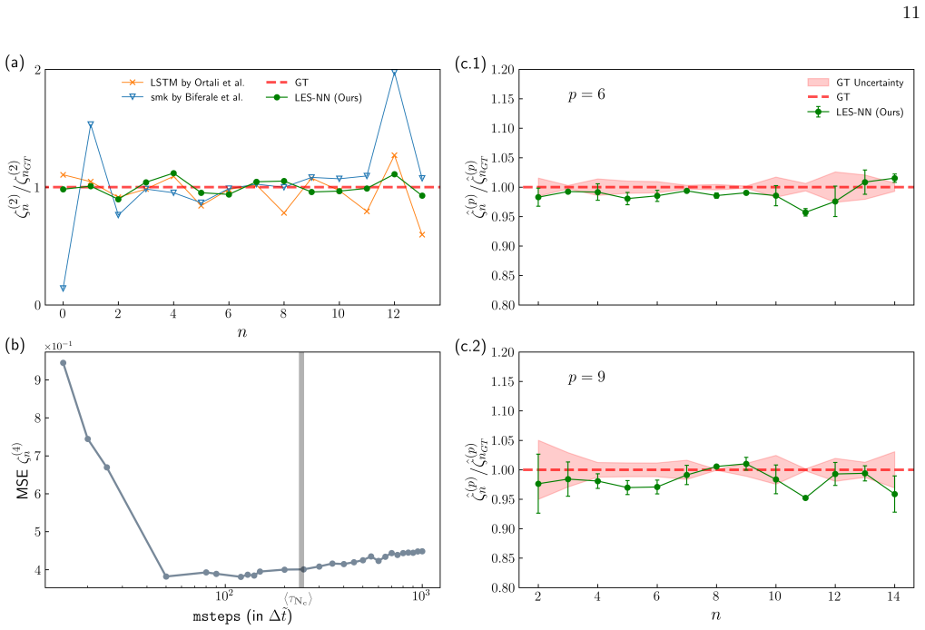
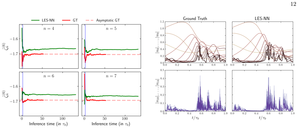
The authors demonstrate that a small MLP, trained for about $50$--$100$ solver steps $(\approx 0.41 \langle \tau_{N_c}\rangle)$, reproduces the fourth to tenth order flatness of the resolved shells, the anomalous scaling exponents $\xi_p$, the Lagrangian structure functions up to order five, and the pdf of the convective flux at the cutoff, correctly capturing backscatter. The trained model remains stable when deployed for times far longer than the training window, and it keeps good accuracy even when the LES time step is increased to $10^{-4}$, i.e., $10{,}000$ times the ground-truth step. Comparisons against an LSTM-based closure and an optimal phenomenological closure show the solver-in-the-loop MLP is most accurate near the cutoff, especially on the local slopes of Eulerian structure functions. The authors interpret the unrolling time as physically meaningful: it should be a fraction of the eddy turnover time of the fastest shell in the loss, because beyond that the ground truth and the model decorrelate and the velocity-based loss becomes uninformative.
Load-bearing premise
The closure assumes that the velocity signals in the three shells just below the cutoff carry enough information to predict the subgrid energy transfer; if the true closure depends on a wider range of scales, the network's input window is insufficient.
Editorial extensions
If this is right
- A simple MLP trained in the loop can reproduce intermittency and rare backscatter events that phenomenological closures miss, without needing a memory-based architecture.
- The unrolling time can be set a priori from the eddy turnover time of the fastest shell in the loss (about $0.41 \langle \tau_{N_c}\rangle$), removing a hyperparameter that is otherwise chosen arbitrarily.
- The trained closure remains stable and accurate when deployed many eddy turnover times past its training window and at LES time steps up to $10^{-4}$ ($10{,}000\times$ the ground-truth step).
- The solver-in-the-loop MLP outperforms both an LSTM and an optimal phenomenological closure on local slopes of structure functions near the cutoff, the most sensitive region for closure error.
- The same differentiable-physics training principle is put forward as a path toward subgrid closures for Navier-Stokes turbulence, where extreme subgrid fluctuations are far harder to capture.
Reading between the lines
- If the three-shell locality assumption survives a systematic convergence test, the computational cost of this closure is essentially independent of Reynolds number, which is not true for 3D LES and would be a decisive practical advantage.
- The physical criterion for the optimal unrolling time may transfer to other chaotic multiscale systems where a differentiable solver is available, giving a first-principles rule for the training horizon instead of trial and error.
- The authors speculate that a flux-based loss would not change the optimal unrolling time; testing that directly would clarify whether the velocity-based loss or the gradient dynamics is the limiting factor.
- The stability of the model beyond its training window suggests the MLP has learned an approximation to the true subgrid transfer operator rather than a one-step correction, raising the possibility of transferring the trained closure to different forcings or cutoffs without retraining.
Editorial analysis
A structured set of objections, weighed in public.
Referee Report
Summary. The paper applies a posteriori (solver-in-the-loop) training to a neural-network closure for the Sabra shell model of turbulence, with the cutoff placed at shell Nc=14 inside the inertial range at extremely high Reynolds number. The closure is an MLP that takes the three shells immediately preceding the cutoff as input and outputs the two shells after the cutoff, which are needed to advance the resolved equations. Training unrolls the differentiable reduced solver for msteps time steps and minimizes a velocity MSE against fully resolved ground truth. The paper reports that the learned closure reproduces flatness up to order 10, Eulerian structure functions and anomalous scaling exponents, Lagrangian structure functions, velocity pdfs, and the subgrid flux pdf including backscatter, and that it outperforms an LSTM and a phenomenological closure on local slopes near the cutoff. It further studies the effect of the unrolling time msteps and concludes that the optimal time in the loop is approximately 0.41 of the eddy turnover time of the fastest shell included in the loss, arguing that this is a physical time scale for the method.
Significance. If the results hold, the paper makes a useful contribution by demonstrating that a simple, memoryless MLP closure trained with a differentiable solver can reproduce strongly non-Gaussian, intermittent statistics of high-Reynolds-number shell-model turbulence, and by proposing a heuristic for choosing the unrolling time. The paper includes several strengths: comparisons against ground truth on held-out test time, chunked error bars on the main statistical observables, a stability test beyond the training horizon, a direct comparison with an LSTM closure and a phenomenological closure, and attention to backscatter in the flux pdf. The central empirical demonstration is not circular, since training uses the ground-truth velocity as a target and evaluation is on different initial conditions and time intervals. However, the generalizability of the method rests on a locality assumption that is asserted but not quantitatively tested, and the proposed time-in-loop rule is fitted post hoc to a single configuration, which limits the strength of the conclusions.
major comments (2)
- [Section III, Eqs. (2)-(3)] The claim that the three shells preceding the cutoff 'is sufficient to close the flux locally' is load-bearing but unsupported. The text states that fewer shells hurt and more do not help, but no figure, table, or quantitative convergence study is provided. Since the MLP maps only (u_{Nc-2}, u_{Nc-1}, u_{Nc}) to (u_{Nc+1}, u_{Nc+2}), the entire method presupposes that the two unresolved shells are an instantaneous function of these three resolved shells. The Sabra dynamics of the unresolved shells are autonomous chaotic ODEs coupled to the resolved state, so memory or nonlocal dependence is not excluded a priori. Please add a systematic input-size study (e.g., 1, 2, 3, 4, or 5 input shells) with the same training and evaluation protocol, and ideally quantify the conditional variance of the true closure given the input state to justify the deterministic MLP mapping.
- [Section IV, Figs. 4(b), 7(b), 10(b)] The conclusion that the optimal time in the loop is around msteps = 100, or about 0.41 of the cutoff-shell eddy turnover time, is derived post hoc from a small set of msteps values, with no error bars and no repeated training runs for each msteps. The ratio 0.41 tau_Nc is therefore a fitted constant, not a parameter-free prediction, and the phrase 'a priori we expect' in Section IV belies the fact that the value is read off from the MSE curves. Furthermore, the study uses a single cutoff shell, a single Reynolds number, and a single forcing protocol, so the proposed physical rule is not demonstrated to generalize. Please provide uncertainty estimates for the optimal msteps, test at least one additional cutoff or Reynolds number, and present the time-in-loop comparison as a post hoc observation rather than an a priori derived law.
minor comments (5)
- [Section III, Eq. (4)] The displayed normalization in Eq. (4) is garbled and does not clearly show the denominator; please reformat the equation so the reader can see exactly how the MSE is normalized.
- [Figure 2 caption] The caption says 'whereas θ denotes an explicit one' using the same symbol as the implicit case; this appears to be a typo and should use distinct notations for the explicit and implicit NN-dependent terms.
- [Section IV, Fig. 5] The pdf of the eddy turnover time tau_n is shown without specifying the units of the horizontal axis; please state whether tau_n is expressed in ground-truth time steps, LES time steps, or absolute time.
- [Section III] The text contains a typo: 'wavenuber' should be 'wavenumber'.
- [Section IV, Fig. 10] The comparison with the LSTM and phenomenological closures is based only on local slopes of the second-order structure function; the paper would be strengthened by stating explicitly that this is one metric among several and by clarifying that the other comparisons are against the ground truth only.
Circularity Check
No significant circularity: the closure is trained on velocity MSE and validated on separate nonlinear statistics, so the reported matches are independent checks.
full rationale
The central demonstration is not circular. The neural closure minimizes the velocity MSE in Eq. (4) over six resolved shells, while the advertised successes—flatnesses (Eq. 5), Eulerian structure functions and anomalous exponents (Eqs. 6 and 9), Lagrangian structure functions (Eq. 11), the cutoff flux pdf (Eq. 15), and local slopes (Eq. 12)—are nonlinear functionals of the generated trajectory that do not enter the loss. The GT and LES-NN are integrated with different time steps, and the test interval (3.31 tau_0) is disjoint from the training interval (1.65 tau_0), so the agreement is an out-of-sample statistical check rather than a recapitulation of the training objective. The three-shell locality ansatz in Section III is an explicit modeling assumption, not a derived result; if it were false the method would be inaccurate, but that is a correctness/limitation issue rather than circularity. The 0.41 <tau_Nc> ratio in Section IV is a post-hoc normalization of the empirically best msteps=100 by the independently measured <tau_Nc>=244; the text explicitly 'looks back' at the fitted MSE curve and does not use that ratio as an input to produce the reported statistics, so no prediction reduces to a fit by construction. Self-citations (Um et al. 2020 for the solver-in-the-loop idea; Biferale et al. 2017 as a baseline) are method attribution and comparison, not load-bearing evidence, and no uniqueness theorem is imported. Overall, the derivation chain is self-contained; no circular step can be exhibited from the paper's equations.
Assumptions & free parameters
free parameters (4)
- Neural network weights =
1e5-4e5 trainable parameters
- Time-in-loop msteps =
100 (optimal for main results; 1, 50, 1000 also tested)
- Optimal time-in-loop ratio 0.41 tau_Nc =
~0.41
- MLP architecture (layer sizes) =
1e5-4e5 parameters, exact layer sizes not specified
assumptions (5)
- domain assumption The Sabra shell model faithfully captures the multiscale energy cascade and intermittency of 3D turbulence
- domain assumption Fully resolved GT with N=40 and nu=1e-12 resolves the dissipative scale (k_N > k_eta)
- ad hoc to paper The three shells preceding the cutoff are sufficient local information to close the flux
- ad hoc to paper Unrolled MSE loss on velocities is a suitable objective for reproducing high-order statistics
- domain assumption RK4 integration with Delta_t=1e-5 for the reduced model is accurate enough for statistical purposes
invented entities (1)
-
Learned neural closure (MLP) mapping three pre-cutoff shells to two post-cutoff shells
Cite this review
Pith. "Pith review of Solver-in-the-loop approach to closure of shell models of turbulence." pith.science (2026). https://pith.science/paper/HNALXNUA
@misc{pith2026241113194,
  author       = {Pith},
  title        = {Pith review of: Solver-in-the-loop approach to closure of shell models of turbulence},
  year         = {2026},
  howpublished = {\url{https://pith.science/paper/HNALXNUA}},
  note         = {Machine review of arXiv:2411.13194}
}
read the original abstract
This work studies an a posteriori data-driven approach (known as solver-in-the-loop) for sub-grid modeling of a shell model for turbulence. This approach takes advantage of the differentiable physics paradigm of deep learning, allowing a neural network model to interact with the differential equation solver over time during the training process. The closure model is, then, naturally exposed to equations-informed input distributions by accounting for prior corrections over the temporal evolution in training. Such a characteristic makes this approach depart from the conventional a priori instantaneous training paradigm and often leads to a more accurate and stable closure model. Our study demonstrates that the closure learned via this a posteriori approach is able to reproduce high-order statistical moments of interest also in closures of high Reynolds number turbulence. Moreover, we investigate the performance of the learned model by experimenting with the effect of unrolling in time, which has remained for the most part unexplored in the literature. Finally, we discuss potential extensions of this approach to Navier-Stokes equations.
Figures


Figures from the paper (9 more)



Reference graph
Works this paper leans on
-
[1]
Frisch, Turbulence: The legacy of A
U. Frisch, Turbulence: The legacy of A. N. Kolmogorov, Cambride University press 10.1017/CBO9781139170666 (1995)
-
[2]
A. Alexakis and L. Biferale, Cascades and transitions in turbulent flows, Physics Reports 10.1016/j.physrep.2018.08.001 (2018)
-
[3]
C. Meneveau and J. Katz, Scale-invariance and turbu- lence models for large-eddy simulation, Annual Review Fluid Mechanics 10.1146/annurev.fluid.32.1.1 (2000)
-
[4]
P. C. M. Lesieur, O. Met´ ais, Large-Eddy Simulations of Turbulence (Cambridge Unversity Press, 2005)
work page 2005
-
[5]
S. B. Pope, Turbulent Flows (IOP Publishing, 2001)
work page 2001
-
[6]
Sagaut, Large Eddy Simulation for Incompressible Flows: An Introduction (Springer, 2006)
P. Sagaut, Large Eddy Simulation for Incompressible Flows: An Introduction (Springer, 2006)
work page 2006
-
[7]
A. A. Mailybaev, Hidden scale invariance of intermittent turbulence in a shell model, Phys. Rev. Fluids6, L012601 (2021)
work page 2021
-
[8]
A. A. Mailybaev and S. Thalabard, Hidden scale invari- ance in navier–stokes intermittency, Philosophical Trans- actions of the Royal Society A: Mathematical, Physical and Engineering Sciences 380, 20210098 (2022)
work page 2022
Show all 43 references
-
[9]
Maulik, O
R. Maulik, O. San, A. Rasheed, and P. Vedula, Sub-grid modelling for two-dimensional turbulence us- ing neural networks, Journal of Fluid Mechanics 10.1017/jfm.2018.770 (2019)
2019 doi
-
[10]
Maulik, O
R. Maulik, O. San, J. D. Jacob, and C. Crick, Sub-grid scale model classification and blending through deep learning, Journal of fluid mechanics https://doi.org/10.1017/jfm.2019.254 (2019)
2019 doi
-
[11]
A. Beck, D. Flad, and C.-D. Munz, Deep neural networks for data-driven LES closure models, Journal of Computa- tional Physics https://doi.org/10.1016/j.jcp.2019.108910 (2019)
2019
-
[12]
Frezat, G
H. Frezat, G. Balarac, J. L. Sommer, R. Fablet, and R. Lguensat, Physical invariance in neural networks for subgrid-scale scalar flux modeling, Physical Review Fluids https://doi.org/10.1103/PhysRevFluids.6.024607 (2021)
2021 doi
-
[13]
Novati, H
G. Novati, H. L. de Laroussilhe, and P. Koumout- sakos, Automating turbulence modelling by multi-agent reinforcement learning, Nature Machine Intelligence 10.1038/s42256-020-00272-0 (2021)
2021 doi
-
[14]
M. Kurz, P. Offenhauser, and A. Beck, Deep reinforce- ment learning for turbulence modeling in large eddy sim- ulations, International Journal of Heat and Fluid Flow 10.1016/j.ijheatfluidflow.2022.109094 (2023)
2023
-
[15]
Biferale, Shell models of energy cascade in turbulence, Annual Review of Fluid Mechanics 35, 441 (2003)
L. Biferale, Shell models of energy cascade in turbulence, Annual Review of Fluid Mechanics 35, 441 (2003)
2003
-
[16]
V. S. L’vov, E. Podivilov, A. Pomyalov, I. Procaccia, and D. Vandembroucq, Improved shell model of turbulence, Physical Review E 58, 1811 (1998)
1998
-
[17]
Hattori, R
Y. Hattori, R. Rubinstein, and A. Ishizawa, Shell model for rotating turbulence, Phys. Rev. E 70, 046311 (2004)
2004
-
[18]
Mingshun and L
J. Mingshun and L. Shida, Scaling behavior of velocity and temperature in a shell model for thermal convective turbulence, Phys. Rev. E 56, 441 (1997)
1997
-
[19]
D. H. Wacks and C. F. Barenghi, Shell model of super- fluid turbulence, Phys. Rev. B 84, 184505 (2011)
2011
-
[20]
Plunian, R
F. Plunian, R. Stepanov, and P. Frick, Shell models of magnetohydrodynamic turbulence, Physics Reports 523, 1 (2013), shell Models of Magnetohydrodynamic Turbu- lence
2013
-
[21]
Benzi, L
R. Benzi, L. Biferale, R. M. Kerr, and E. Trovatore, Heli- cal shell models for three-dimensional turbulence, Phys. Rev. E 53, 3541 (1996)
1996
-
[22]
M. H. Jensen, G. Paladin, and A. Vulpiani, Shell model for turbulent advection of passive-scalar fields, Phys. Rev. A 45, 7214 (1992)
1992
-
[23]
A. A. Mailybaev, Spontaneously stochastic solutions in one-dimensional inviscid systems, Nonlinearity 29, 2238 (2016)
2016
-
[24]
Bandak, A
D. Bandak, A. A. Mailybaev, G. L. Eyink, and N. Gold- enfeld, Spontaneous stochasticity amplifies even thermal noise to the largest scales of turbulence in a few eddy turnover times, Phys. Rev. Lett. 132, 104002 (2024)
2024
-
[25]
Constantin, B
P. Constantin, B. Levant, and E. S. Titi, Regularity of inviscid shell models of turbulence, Phys. Rev. E 75, 016304 (2007)
2007
-
[26]
Daumont, T
I. Daumont, T. Dombre, and J.-L. Gilson, Instanton cal- culus in shell models of turbulence, Phys. Rev. E62, 3592 (2000)
2000
-
[27]
Vinuesa and S
R. Vinuesa and S. L. Brunton, Enhancing computational fluid dynamics with machine learning, Nature Computa- tional Science 2, 358 (2022)
2022
-
[28]
C. Cho, J. Park, and H. Choi, A recursive neural- network-based subgrid-scale model for large eddy simu- lation: application to homogeneous isotropic turbulence, Journal of Fluid Mechanics 1000, A76 (2024)
2024
-
[29]
K. Duraisamy, Perspectives on machine learning- augmented Reynolds-averaged and large eddy simu- lation models of turbulence, Physical Review Flu- ids 6, https://doi.org/10.1103/PhysRevFluids.6.050504 (2019)
2019 doi
-
[30]
Biferale, A
L. Biferale, A. A. Mailybaev, and G. Parisi, Optimal sub- grid scheme for shell models of turbulence, Physical Re- view E 95, 10.1103/physreve.95.043108 (2017)
2017 doi
-
[31]
Ortali, A
G. Ortali, A. Corbetta, G. Rozza, and F. Toschi, Nu- merical proof of shell model turbulence closure, Physical Review Fluids 7, 10.1103/physrevfluids.7.l082401 (2022)
2022 doi
-
[32]
J. D. Lemos and A. A. Mailybaev, Data-based approach for time-correlated closures of turbulence models, Physi- cal Review E 109, 10.1103/physreve.109.025101 (2024)
2024 doi
-
[33]
K. Um, R. Brand, Y. Fei, P. Holl, and N. Thuerey, Solver- in-the-loop: Learning from differentiable physics to inter- act with iterative pde-solvers, Advances in Neural Infor- mation Processing Systems (2020)
2020
-
[34]
List, L.-W
B. List, L.-W. Chen, K. Bali, and N. Thuerey, How temporal unrolling supports neural physics simulators (2024), arXiv:2402.12971 [cs.LG]
2024 arXiv
-
[35]
Fukushima, Neocognitron: A self-organizing neural network model for a mechanism of pattern recognition unaffected by shift in position, Biological Cybernetics36, 193–202 (1980)
K. Fukushima, Neocognitron: A self-organizing neural network model for a mechanism of pattern recognition unaffected by shift in position, Biological Cybernetics36, 193–202 (1980)
1980
-
[36]
Sirignano, J
J. Sirignano, J. F. MacArt, and J. B. Freund, DPM: A deep learning PDE augmentation method with applica- tion to large-eddy simulation, Journal of Computational Physics 423, 109811 (2020)
2020
-
[37]
Shankar, V
V. Shankar, V. Puri, R. Balakrishnan, R. Maulik, and V. Viswanathan, Differentiable physics-enabled closure modeling for Burgers’ turbulence, Machine Learning: Science and Technology 4, 015017 (2023). 14
2023
- [38]
-
[39]
Cheng and D
B. Cheng and D. M. Titterington, Neural networks: A review from a statistical perspective, Statistical Science 10.1214/ss/1177010638 (1994)
1994
-
[40]
A. N. Kolmogorov, The local structure of turbulence in incompressible viscous fluid for very large Reynolds num- bers, Proc. Math. Phys. Eng. Sci 434, 9 (1991)
1991
-
[41]
She and E
Z.-S. She and E. Leveque, Universal scaling laws in fully developed turbulence, Physical Review Letters 72, 336 (1994)
1994
-
[42]
Hochreiter and J
S. Hochreiter and J. Schmidhuber, Long short-term mem- ory, Neural Computation 9, 1735 (1997)
1997
-
[43]
R. M. Larsen and T. Shpeisman, Tensorflow graph opti- mizations (2019)
2019
Reviewed August 12, 2026 · model on record in the stance chip above.
Discussion (0). Continue with ORCID to comment.