REVIEW 3 major objections 4 minor 1 cited by
Blurring the Busse balloon: Patterns in a stochastic Klausmeier model
T0 review · 3 major / 4 minor · reviewed 2026-08-12 · deepseek-v4-flash
Pith's one-line read Stochastic forcing blurs the boundary of the deterministic Busse balloon in a dryland vegetation model.
desk verdict Noise blurs the Busse balloon in the Klausmeier model, but the pulse-counting definition of exit time needs a robustness check before I'd trust the quantitative claims. read the letter →
The pith
A machine-rendered reading of the paper's core claim, the machinery that carries it, and where it could break.
The reading
What carries the argument
Busse balloon: the region in parameter space of deterministically stable periodic wave numbers, traced by numerical continuation. First exit time: the first time the pulse number changes, estimated by averaging over many noise realizations; it mimics deterministic stability in the stochastic setting. Local wave number: the predominant mode of a Gaussian-windowed Fourier transform with width $\ell=50$; it captures both the number of pulses and their spatial distribution. The pulse number itself is counted by smoothing the solution and locating extrema with a prominence threshold, a heuristic that defines when destabilization is said to occur.
What would settle it
Run the $a=2.0$, $\sigma=0.25$ stochastic simulations with the pulse-counting thresholds varied (smoothing width and prominence) and check whether wave number 38 still has a longer average first exit time than wave numbers 23 and 24; if the ordering reverses, the claimed blurring is an artifact of the pulse-counting definition.
Extended reading notes
Core claim
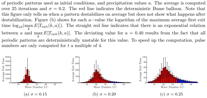
The paper studies the one-dimensional stochastic Klausmeier model (1.1), a reaction-diffusion system for dryland vegetation with multiplicative noise in the mortality rate. It claims that stochastic forcing does not simply destroy the deterministic Busse balloon but blurs its boundary: for fixed rainfall $a=2.0$ and noise $\sigma=0.25$, the average first exit time of the deterministically unstable wave number 38 exceeds that of the deterministically stable wave numbers 23 and 24, so the observed boundary of the balloon is no longer sharp. The blurring is controlled by position within the balloon and noise level: patterns in the centre survive longest, exit times grow exponentially in the rainfall parameter $a$ and obey a power law in $\sigma$, and the boundary sharpens again in the limit $\sigma\to 0$ and $T_{\max}\to\infty$. The paper also introduces local wave numbers to describe what solutions look like after destabilization, showing that typical stochastic solutions are patchworks of different local wave numbers rather than a single global mode.
Load-bearing premise
The definition of first exit time rests on a heuristic pulse-counting procedure (Gaussian smoothing width 64 gridpoints, prominence threshold 0.3); if a different threshold is used, measured exit times and the reported blurring of the balloon boundary could change.
Editorial extensions
If this is right
- Within the stochastic model, patterns near the centre of the deterministic Busse balloon are the most persistent, but the deterministic boundary loses its predictive power for observability once noise is present.
- Reducing the noise intensity increases exit times most strongly in the balloon's interior, so the sharp deterministic boundary is recovered only in the double limit $\sigma\to 0$ and $T_{\max}\to\infty$.
- Typical stochastic solutions are not close to a single periodic pattern: the stationary distribution of local wave numbers is spread across the balloon and shifts with $a$ and $\sigma$.
- Because exit times are exponentially sensitive to rainfall and power-law sensitive to noise, the relevant pattern persistence timescale can change by orders of magnitude within the parameter range studied.
- The three measures of stability peak at different wave numbers (31 for exit time, 30 for deterministic selection, 28 for stationary distribution), so 'most stable' depends on which observable is used.
Reading between the lines
- If the blurring mechanism is generic, the same pulse-deletion route should blur Busse balloons in other stochastic reaction-diffusion systems, such as Swift-Hohenberg or Gray-Scott; a direct test would be to repeat the exit-time scan for those models.
- The measured exponential-in-$a$ and power-law-in-$\sigma$ relations for exit times could be turned into a scaling law for pattern persistence in dryland vegetation, once dimensional rainfall and disturbance intensity are calibrated.
- A Markov chain on pulse numbers with transition rates estimated from short stochastic runs could convert the blurred balloon into a quantitative prediction of how fast patterns degrade, although the paper notes the state definition is delicate.
- In two-dimensional stripe patterns, the noise is correlated along the stripe direction in the present one-dimensional setup; in true two dimensions, local defects may nucleate differently, so the blurring could appear at lower noise levels.
Editorial analysis
A structured set of objections, weighed in public.
Referee Report
Summary. The paper studies the one-dimensional stochastic Klausmeier model (1.1) with multiplicative noise in the vegetation mortality. It defines the first exit time Texit as the first time the number of pulses changes, and it introduces local Fourier transforms to assign local wavenumbers to transient and noisy patterns. Numerical experiments show that average exit times vary strongly with rainfall a, wavenumber k, and noise intensity sigma, and that for a=2 and sigma=0.25 the mean exit time at k=38 exceeds that at k=23 and 24 even though k=38 lies outside the deterministic Busse balloon. The authors also compute long-time local-wavenumber distributions, which concentrate around the middle of the balloon, and conclude that stochasticity blurs the boundary of the deterministic Busse balloon while the boundary becomes sharp again in the limit sigma -> 0 and Tmax -> infinity.
Significance. The manuscript addresses a timely question: whether the deterministic Busse balloon remains a useful stability concept under stochastic forcing. The proposed tools, average first exit times and local wavenumber distributions, are natural and well motivated, and the numerical experiments are direct simulations rather than fitted outputs, which avoids circularity. If the central reversal in Figure 8c is robust, the paper gives a concrete, falsifiable statement about stochastic destabilization in a canonical ecological model, and the open-source scripts on GitHub are a strength for reproducibility. The comparison with empirical Busse balloons from Bastiaansen et al. is a useful sanity check. However, the robustness of the pulse-counting definition and the unsupported stationarity label for sigma=0.2 are load-bearing gaps that need to be addressed before the claims can be accepted.
major comments (3)
- [Section 2.3, Appendix A.3, Figure 8c] The central reversal in Figure 8c depends on the pulse-counting detector: Texit is the first time the pulse number changes, and in Appendix A.3 the pulse number is obtained by smoothing u with a Gaussian of width 64 gridpoints and counting extrema with MinProminence 0.3, a procedure the authors themselves call heuristic in Section 2.3. Because k=38 has a much shorter wavelength than k=23 or 24, a fixed smoothing width and prominence threshold can have wavenumber-dependent detection lag: a dying short-wavelength pulse at k=38 may be registered as present for a different length of time than a dying long-wavelength pulse, purely because of the detector. The paper provides no test that the ordering E[Texit(38)] > E[Texit(23)], E[Texit(24)] survives variation of the smoothing width or MinProminence, or comparison with a different destabilization criterion. Please add a robustness study of this specific reversal, for example by recomputing Texit with smoothing widths of 32 and 128 gridpoints and MinProminence values of 0.15 and 0.6, and by checking the same ordering with a criterion based on the local wavenumber distribution or on amplitude decay.
- [Section 3.2, Appendix A.4, Figures 9b and 10c] The claim that Figures 9b and 10c show stationary distributions is not supported by the paper's own convergence test. Section 3.2 says that Appendix A.4 validates stationarity, but Appendix A.4 explicitly states that for sigma=0.2 two different initial conditions lead to different distributions at T=Tmax=10^4 and that the simulations have not yet reached the stationary distribution. Nevertheless, Figure 9b is labeled as a stationary distribution for sigma=0.2, and Figure 10c uses the same object to compare stability measures. This internal inconsistency affects the observability conclusions. Please either restrict the stationarity claim to sigma=0.25, or present the sigma=0.2 results as finite-time long-time distributions with a quantitative convergence assessment, and state whether the comparison in Figure 10 changes when only verified stationary cases are used.
- [Figure 8c and Section 3.1] Figure 8c reports E[Texit] over 50 realizations and displays the standard deviation of the exit times, but the central claim that the mean exit time at k=38 exceeds those at k=23 and 24 is not accompanied by a standard error, a confidence interval, or a pairwise significance test. With heavy-tailed exit-time data and only 50 runs, the observed reversal may be within sampling error, and the caption's note that standard deviations are added to highlight the high variability makes this concern concrete. Additionally, Texit is right-censored at Tmax, so the fraction of runs that reached Tmax for each k must be reported, since censoring biases the estimated mean differently across wavenumbers. Please provide mean uncertainties and censoring counts for the bars in Figure 8c, and test the ordering of the means.
minor comments (4)
- [Figure 9 caption] The caption of Figure 9 states Tmax=2500, while Section 3.2 states Tmax=10^4 for the same computations; please reconcile the two values.
- [Figure A.4 and Figure 7b] Figure A.4 claims a power-law relation Texit ~ sigma^alpha with alpha approximately 10 based on a visual log-log fit, and Figure 7b claims an exponential relation between a and the maximum exit time from a straight-line fit; report the number of data points, regression standard errors, and residual diagnostics for both fits, and state how the a=0.40 outlier in Figure 7b is treated.
- [Appendix A.3] Appendix A.3 mentions a moving median in time to filter short fluctuations but does not specify its window length; since the pulse number and thus Texit can depend on this parameter, please give the value used.
- [Section 2.2] The local Fourier transform window width ell=50 is fixed a priori; a brief discussion of the sensitivity of the local wavenumber statistics to ell would help readers assess the observability claims.
Circularity Check
No circularity: the stochastic blurring claim is a direct numerical measurement compared against an independently computed Busse balloon.
full rationale
The paper's central quantities are direct simulation outputs, not fitted inputs renamed as predictions. Texit is defined as the first time the measured pulse number changes (Section 2.3) and is estimated by repeated numerical integration of the stochastic PDE (1.1); the deterministic Busse balloon boundary in Figure 1 is computed independently with the continuation software auto-07p [10]. The blurring conclusion in Section 3.1 is therefore an empirical comparison between two independently generated objects. The scaling laws in Figure 7b and Figure A.4 are descriptive fits to the simulated exit times and are not used to define Texit, so no fitted parameter is called a prediction. The local wave number method follows [38] and the numerical integrator follows [22]; both are methodological citations with independent content, and self-citations such as [6] and [32] supply only a parameter value or contextual comparison. The acknowledged heuristic in pulse counting ('determining the pulse number in a simulation is in some sense heuristic as different settings in the procedure may result in different pulse numbers', Section 2.3; smoothing details in Appendix A.3) is a measurement caveat, not a circular reduction: no equation defines the Busse balloon boundary in terms of Texit, and the measured ordering in Figure 8c is not equal by construction to the deterministic stability classification.
Assumptions & free parameters
free parameters (5)
- Local Fourier transform window width ell =
50
- Pulse detection smoothing parameters =
Gaussian width 64 gridpoints, MinProminence 0.3
- Noise spatial correlation length xi =
0.1
- Power-law exponent alpha in Texit ~ sigma^alpha =
~10
- Exponential decay rate of max exit time vs a =
not stated (slope of line in Fig 7b)
assumptions (4)
- domain assumption The stochastic Klausmeier model (1.1) with Ito multiplicative noise is an adequate representation of dryland vegetation dynamics.
- domain assumption The deterministic Busse balloon computed by continuation (pde2path) correctly identifies stable periodic patterns of the deterministic model.
- domain assumption Spatial discretization and time-stepping scheme (A.2) accurately approximate the SPDE solutions, including the noise term.
- ad hoc to paper The distribution of local wave numbers at Tmax is stationary for sigma=0.2 and a up to 2.5, even though A.4 shows non-convergence for sigma=0.2.
Cite this review
Pith. "Pith review of Blurring the Busse balloon: Patterns in a stochastic Klausmeier model." pith.science (2026). https://pith.science/paper/N43RZTQE
@misc{pith2026241113238,
  author       = {Pith},
  title        = {Pith review of: Blurring the Busse balloon: Patterns in a stochastic Klausmeier model},
  year         = {2026},
  howpublished = {\url{https://pith.science/paper/N43RZTQE}},
  note         = {Machine review of arXiv:2411.13238}
}
read the original abstract
We investigate (in)stabilities of periodic patterns under stochastic forcing in reaction-diffusion equations exhibiting a so-called Busse balloon. Specifically, we used a one-dimensional Klausmeier model for dryland vegetation patterns. Using numerical methods, we can accurately describe the transient dynamics of the stochastic solutions and compare several notions of stability. In particular, we show that stochastic stability heavily depends on the model parameters, the intensity of the noise and the location of the wavenumber of the periodic pattern within the deterministic Busse balloon. Furthermore, the boundary of the Busse balloon becomes blurred under the stochastic perturbations.
Figures


Figures from the paper (8 more)




Forward citations
Cited by 1 Pith paper
-
A flow-kick model of dryland vegetation patterns: the impact of rainfall variability on resilience
In a flow-kick model of dryland vegetation, random storm timing and depth at fixed mean annual rainfall narrows the precipitation window in which banded vegetation patterns form, compared to periodic rainfall.
Reference graph
Works this paper leans on
-
[1]
B. M. Arani, S. R. Carpenter, L. Lahti, E. H. Van Nes and M. Scheffer (2021), Exit time as a measure of ecological resilience. Science 372(6547), eaay4895
work page 2021
-
[2]
A. Asch, M. Avery, A. Cortez and A. Scheel (2024), Slow passage through the Busse balloon– predicting steps on the Eckhaus staircase. European Journal of Applied Mathematics pp. 1–26
work page 2024
-
[3]
M. E. Assessment (2003), Ecosystems and Human Well-being; A Framework for Assessment . Island Press
work page 2003
-
[4]
R. Bastiaansen, P. Carter and A. Doelman (2019), Stable planar vegetation stripe patterns on sloped terrain in dryland ecosystems. Nonlinearity 32(8), 2759
work page 2019
-
[5]
R. Bastiaansen and A. Doelman (2019), The dynamics of disappearing pulses in a singularly perturbed reaction–diffusion system with parameters that vary in time and space. Physica D: Nonlinear Phenomena 388, 45–72
work page 2019
-
[6]
R. Bastiaansen, O. Ja ¨ ıbi, V. Deblauwe, M. B. Eppinga, K. Siteur, E. Siero, S. Mermoz, A. Bouvet, A. Doelman, and M. Rietkerk (2018), Multistability of model and real dryland ecosystems through spatial self-organization. Proceedings of the National Academy of Sciences 115(44), 11256–11261
work page 2018
-
[7]
Busse (1978), Non-linear properties of thermal convection
F. Busse (1978), Non-linear properties of thermal convection. Reports on Progress in Physics 41(12), 1929
work page 1978
-
[8]
J. Couwenberg and H. Joosten (2005), Self-organization in raised bog patterning: the origin of microtope zonation and mesotope diversity. Journal of Ecology pp. 1238–1248
work page 2005
Show all 38 references
-
[9]
Deblauwe, N
V. Deblauwe, N. Barbier, P. Couteron, O. Lejeune and J. Bogaert (2008), The global biogeo- graphy of semi-arid periodic vegetation patterns. Global Ecology and Biogeography 17(6), 715–723
2008
-
[10]
Doedel, A
E. Doedel, A. Champneys, T. Fairgrieve, Y. Kuznetsov, B. Sandstede, and X. Wang (1998), AUTO 97:Continuation and bifurcation software for ordinary differential equations. Technical report, Concordia University
1998
-
[11]
Eigentler and J
L. Eigentler and J. A. Sherratt (2020), Effects of precipitation intermittency on vegetation patterns in semi-arid landscapes. Physica D: Nonlinear Phenomena 405, 132396
2020
-
[12]
Eppinga, P
M. Eppinga, P. de Ruiter, M. Wassen and M. Rietkerk (2009), Nutrients and Hydrology Indicate the Driving Mechanisms of Peatland Surface Patterning. The American Naturalist 173(6), 803–818
2009
-
[13]
D. R. Foster, G. A. King, P. H. Glaser and H. E. Wright (1983), Origin of string patterns in boreal peatlands. Nature 306(5940), 256–258
1983
-
[14]
Gandhi, S
P. Gandhi, S. Bonetti, S. Iams, A. Porporato and M. Silber (2020), A fast–slow model of banded vegetation pattern formation in drylands. Physica D: Nonlinear Phenomena 410, 132534
2020
-
[15]
Gandhi, L
P. Gandhi, L. Liu and M. Silber (2023), A pulsed-precipitation model of dryland vegetation pattern formation. SIAM Journal on Applied Dynamical Systems 22(2), 657–693
2023
-
[16]
Gilad, J
E. Gilad, J. von Hardenberg, A. Provenzale, M. Shachak and E. Meron (2004), Ecosystem Engineers: From Pattern Formation to Habitat Creation. Physical Review Letters 93, 1–4. 14
2004
-
[17]
Grafke and E
T. Grafke and E. Vanden-Eijnden (2019), Numerical computation of rare events via large deviation theory. Chaos: An Interdisciplinary Journal of Nonlinear Science 29(6)
2019
-
[18]
Hille Ris Lambers, M
R. Hille Ris Lambers, M. Rietkerk, F. V. D. Bosch, H. H. T. Prins and H. D. Kroon (2001), Vegetation Pattern Formation in Semi-Arid Grazing Systems. Ecology 82, 50–61
2001
-
[19]
K¨ astner, R
K. K¨ astner, R. C. Van de Vijsel, D. Caviedes-Voulli` eme and C. Hinz (2024), A scale-invariant method for quantifying the regularity of environmental spatial patterns. Ecological Complexity 60, 101104
2024
-
[20]
C. A. Klausmeier (1999), Regular and irregular patterns in semiarid vegetation. Science 284(5421), 1826–1828
1999
-
[21]
Kondo and T
S. Kondo and T. Miura (2010), Reaction-diffusion model as a framework for understanding biological pattern formation. Science 329(5999), 1616–1620
2010
-
[22]
G. J. Lord, C. E. Powell and T. Shardlow (2014), An introduction to computational stochastic PDEs. Cambridge University Press
2014
-
[23]
Macfadyen (1950), Vegetation patterns in the semi-desert plains of British Somaliland
W. Macfadyen (1950), Vegetation patterns in the semi-desert plains of British Somaliland. Geographical Journal 116, 199–211
1950
-
[24]
Martinez-Garcia, C
R. Martinez-Garcia, C. Cabal, J. M. Calabrese, E. Hern´ andez-Garc ´ ıa, C. E. Tarnita, C. L´ opez, and J. A. Bonachela (2023), Integrating theory and experiments to link local mechanisms and ecosystem-level consequences of vegetation patterns in drylands. Chaos, Solitons & Fr...
2023
-
[25]
J. D. Murray (2003), Mathematical Biology II: Spatial Models and Biomedical Applications , Vol. 18 of Interdisciplinary Applied Mathematics . Springer New York
2003
-
[26]
Rademacher, B
J. Rademacher, B. Sandstede and A. Scheel (2007), Computing absolute and essential spectra using continuation. Physica D: Nonlinear Phenomena 229, 166–183
2007
-
[27]
Rietkerk, R
M. Rietkerk, R. Bastiaansen, S. Banerjee, J. van de Koppel, M. Baudena, and A. Doelman (2021), Evasion of tipping in complex systems through spatial pattern formation. Science 374(6564)
2021
-
[28]
Scheffer, J
M. Scheffer, J. Bascompte, W. Brock, V. Brovkin, S. Carpenter, V. Dakos, H. Held, E. van Nes, M. Rietkerk, and G. Sugihara (2009), Early-warning signals for critical transitions.Nature 461, 53–59
2009
-
[29]
J. A. Sherratt (2013), History-dependent patterns of whole ecosystems. Ecological Complexity 14, 8–20
2013
-
[30]
J. A. Sherratt and G. J. Lord (2007), Nonlinear dynamics and pattern bifurcations in a model for vegetation stripes in semi-arid environments. Theoretical population biology 71(1), 1–11
2007
-
[31]
Siero (2018), Nonlocal grazing in patterned ecosystems
E. Siero (2018), Nonlocal grazing in patterned ecosystems. Journal of Theoretical Biology 436, 64–71
2018
-
[32]
Siteur, E
K. Siteur, E. Siero, M. B. Eppinga, J. D. Rademacher, A. Doelman, and M. Rietkerk (2014), Beyond Turing: The response of patterned ecosystems to environmental change. Ecological Complexity 20, 81–96
2014
-
[33]
Uecker (2022), Continuation and bifurcation in nonlinear PDEs–Algorithms, applications, and experiments
H. Uecker (2022), Continuation and bifurcation in nonlinear PDEs–Algorithms, applications, and experiments. Jahresbericht der Deutschen Mathematiker-Vereinigung pp. 1–38. 15
2022
-
[34]
Uecker, D
H. Uecker, D. Wetzel and J. D. Rademacher (2014), pde2path-A Matlab package for continu- ation and bifurcation in 2D elliptic systems. Numerical Mathematics: Theory, Methods and Applications 7(1), 58–106
2014
-
[35]
van de Koppel, J
J. van de Koppel, J. C. Gascoigne, G. Theraulaz, M. Rietkerk, W. M. Mooij, and P. M. Herman (2008), Experimental evidence for spatial self-organization and its emergent effects in mussel bed ecosystems. Science 322(5902), 739–742
2008
-
[36]
van de Koppel, M
J. van de Koppel, M. Rietkerk, N. Dankers and P. Herman (2005), Scale-dependent feedback and regular spatial patterns in young mussel beds. The American naturalist 165(3), E66–77
2005
-
[37]
van der Stelt, A
S. van der Stelt, A. Doelman, G. Hek and J. D. Rademacher (2013), Rise and fall of periodic patterns for a generalized Klausmeier–Gray–Scott model. Journal of Nonlinear Science 23, 39–95
2013
-
[38]
Vi˜ nals, E
J. Vi˜ nals, E. Hern´ andez-Garc ´ ıa, M. San Miguel and R. Toral (1991), Numerical study of the dynamical aspects of pattern selection in the stochastic Swift-Hohenberg equation in one dimension. Physical Review A 44(2), 1123. A Appendix A.1 Computation of the most unstable m...
1991
Reviewed August 12, 2026 · model on record in the stance chip above.
Discussion (0). Continue with ORCID to comment.