REVIEW 3 major objections 5 minor 1 cited by
Abstracted Model Reduction: A General Framework for Efficient Interconnected System Reduction
T0 review · 3 major / 5 minor · reviewed 2026-08-12 · deepseek-v4-flash
Pith's one-line read This paper proposes abstracted model reduction: substitute a low-order stand-in for the environment before applying structure-preserving reduction, and keep most of the closed-loop accuracy at a fraction of the cost.
desk verdict Solid framework paper: abstracted reduction is a real step forward for structure-preserving reduction, but the advertised automatic guarantee needs the full environment model, so it does not cover the unknown-environment case. read the letter →
The pith
A machine-rendered reading of the paper's core claim, the machinery that carries it, and where it could break.
The reading
What carries the argument
The central object is the abstracted interconnection $F_l(\hat{F}, \Sigma)$, obtained by replacing the environment $E(s)$ with a low-order $\hat{E}(s)$ and augmenting it with weighting matrices $G_u$ and $G_y$. The paper shows that $\hat{\Sigma}$ can be recovered from the augmented closed-loop error $\Lambda_F$ through an upper LFT inversion, and that the final error satisfies $\Lambda_C = F_u(N, \operatorname{diag}(\Lambda_{E,22}, \tilde{\Lambda}_F, \Lambda_{E,22}))$, where $M = \Sigma(I - E_{22}\Sigma)^{-1}$ is the closed-loop map of the true system. This identity carries the argument: it separates the error budget into an abstraction part and a reduction part, allows the robust-performance optimization of Theorems 3 and 4, and justifies substituting the original environment after reduction.
What would settle it
Construct an example where the environment abstraction $\hat{E}$ satisfies the $\Lambda_{E,22}$ bound but is deliberately poor in $\hat{E}_{11}, \hat{E}_{12}, \hat{E}_{21}$; the paper's Theorem 1 says only $\Lambda_{E,22}$ enters $\Lambda_C$ directly, but $\Lambda_F$ depends on all of $\hat{E}$, so a large measured $\Lambda_C$ would show that the off-diagonal abstraction error cannot be ignored.
Extended reading notes
Core claim
The core discovery is that the environment of a subsystem acts mainly as a weighting that determines which subsystem dynamics matter for the interconnected response, and that this weighting can be replaced by a low-order abstraction without losing the essential information. Concretely, the paper expresses the total interconnected reduction error as $\Lambda_C = F_u(N, \operatorname{diag}(\Lambda_{E,22}, \tilde{\Lambda}_F, \Lambda_{E,22}))$, with $M = \Sigma(I - E_{22}\Sigma)^{-1}$, showing that only the $22$-block of the abstraction error enters this relation directly, while the reduction error is measured through the augmented closed loop $F_l(\hat{F}, \Sigma)$. This error relation is turned into a certificate: if the abstraction and reduction errors stay within frequency-weighted bounds that satisfy a scaled structured-singular-value condition, then the reduced interconnected model is stable and meets the prescribed accuracy specification. The numerical demonstration shows that reducing the environment by over 80% does not degrade the accuracy of the reduced interconnected model, which is the concrete sense in which the abstraction is sufficient.
Load-bearing premise
The formal error and stability guarantees require that the full, true environment model $E(s)$ is available before reduction, so the certificate does not cover the modular-design situation in which only a rough environment model is known.
Editorial extensions
If this is right
- Structure-preserving reduction becomes computationally feasible for interconnected systems whose environment order dominates, because the cost drops from $(n_E+n_\Sigma)^c$ to $(r_E+n_\Sigma)^c$.
- A low-order abstraction of the environment is sufficient to indicate which subsystem dynamics to retain: in the case study, reducing the environment by over 80% did not significantly degrade the reduced interconnected model.
- User-specified frequency-dependent accuracy specifications can be met automatically by allocating error budgets between abstraction and reduction, with stability preserved when a true environment model is available.
- Abstracted reduction is compatible with any structure-preserving reduction method, so improved reduction methods can be plugged into the framework without changing the abstraction step.
- In the benchmark, abstracted closed-loop balanced reduction achieved $\|\Lambda_C\|_2 = 7.70\times10^{-6}$ in 39 seconds, close to the full structure-preserving result $6.24\times10^{-6}$ in 231 seconds.
Reading between the lines
- The error-relation theorem suggests that the off-diagonal blocks $\hat{E}_{11}, \hat{E}_{12}, \hat{E}_{21}$ of the abstraction only influence the final error through the reduction step; a natural testable extension is to check whether cheaply approximating only $E_{22}$ is enough when the reduction method is insensitive to the other blocks.
- Because the certificate requires the true environment, the practical modular-design setting discussed in Remark 1 would need a separate validation procedure, for example bracketing the unknown environment with a family of models and checking the error bound over that family.
- The $\beta$ trade-off suggests an automated hyperparameter selection based on estimated reduction cost, rather than the manual tuning currently needed to balance $r_E$ and $r_\Sigma$.
- If abstraction is viewed as a learned or data-driven surrogate, the same framework could allow reduction when only input-output data of the environment is available, though the formal error analysis would need replacing.
Editorial analysis
A structured set of objections, weighed in public.
Referee Report
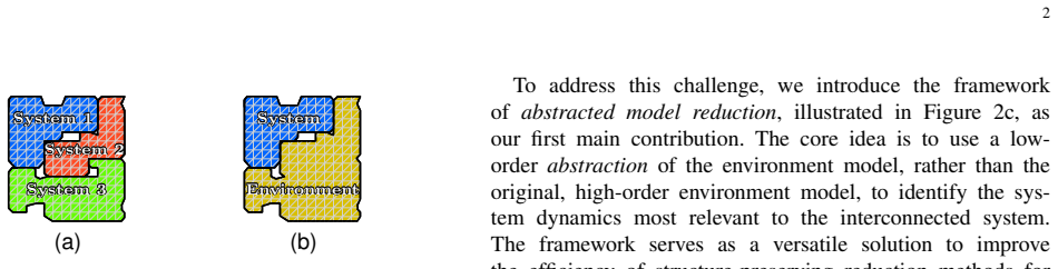
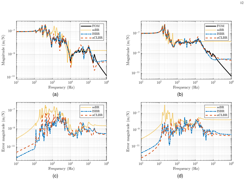
Summary. The paper introduces "abstracted model reduction," a framework for reducing a subsystem of an interconnected system while it is coupled to a low-order abstraction of its environment rather than to the full environment. Algorithm 1 performs four steps: abstract E to \hat{E}, augment the abstraction to form \hat{F}, apply a structure-preserving reduction method to Fl(\hat{F},\Sigma), and finally substitute the original E back to obtain Fl(E,\hat{\Sigma}). Section IV derives an LFT expression for the coupled error \Lambda_C = Fl(E,\hat{\Sigma}) - Fl(E,\Sigma) in terms of the abstraction error \Lambda_{E,22} and the reduction error \tilde{\Lambda}_F, namely \Lambda_C = Fu(N,\mathrm{diag}(\Lambda_{E,22},\tilde{\Lambda}_F,\Lambda_{E,22})) with nominal model N in (16). Using \mu-analysis and the authors' prior robust-performance results, Theorem 2 and Corollary 1 convert a prescribed bound on \Lambda_C into bounds on the two error sources, and Theorem 3 / Theorem 4 formulate optimization problems for allocating these error budgets. Algorithm 2 is the resulting "robust abstracted reduction" routine with automatic order selection. The paper evaluates both frameworks on a 2136-th-order lithography structural-dynamics model with five components. In the fixed-order comparison, abstracted closed-loop balanced reduction (aCLBR) achieves \|\Lambda_C\|_2 = 7.70e-6 in 39 s, close to full ISBR (6.24e-6 in 231 s) and much better than subsystem balanced reduction (2.56e-5 in 19 s).
Significance. If the central claims hold, the framework is a genuinely useful bridge between cheap open-loop reduction and expensive structure-preserving reduction: it gives a principled way to choose a low-order environment abstraction, relates abstraction and reduction errors to the final interconnected-system error through a clean LFT formula, and demonstrates on a realistic industrial model that most of the accuracy benefit of structure-preserving reduction can be retained at a small fraction of its cost. The use of \mu-analysis is appropriate, and the paper is notably honest: Remark 1 acknowledges that the formal error analysis requires the true environment model, and Section VI-B transparently reports the conservatism of the robust routine. The empirical comparison in Table II is informative, and the 80% environment-reduction result is a useful, falsifiable statement about the motivating application. The main limitation, discussed below, is that the strongest advertised guarantee does not cover the modular/unknown-environment scenario that motivates the framework in Section II-B; this is a scope restriction rather than an internal inconsistency.
major comments (3)
- [Sec. II-B, II-C, Remark 1, Algorithm 2] The robust guarantee advertised in the abstract and Section V is conditional on having the true environment E, not on having only a preliminary model \hat{E}. Algorithm 2 and Theorem 3 construct the nominal model N(s) in (16), which contains M(s)=\Sigma(I-E_{22}\Sigma)^{-1} from (17); this is the exact closed-loop map of the true E. Similarly, verifying the budgets \Lambda_{E,22}\in \overline{\Lambda}_{E,22} and \tilde{\Lambda}_F\in \overline{\Lambda}_F requires evaluating the full-order interconnection before reduction. Remark 1 explicitly concedes that if only a preliminary \hat{E} is known, "the formal error analysis of Section IV can not be applied." Consequently, Algorithm 2 does not deliver a guarantee for the modular design scenario described in Section II-B, where E is typically unavailable or only a rough estimate. The abstract and conclusions should be qualified to state that the automatic stability/accuracy guarantee applies when E is already known and evaluable, and the paper should either extend the analysis to environment-model uncertainty or clearly mark this as a key open problem. The empirical Table II comparison is not affected, but the strongest advertised deliverable is.
- [Sec. IV, Lemma 2 / Theorem 1 and Sec. VI-A] The formal error analysis requires square invertible weighting matrices Gu and Gy, but the main empirical comparison of the general framework uses Gu=Gy=O. Lemma 2 states the inversion result for "square, invertible matrices Gu and Gy," yet Theorem 1, which follows immediately, does not restate this assumption and defines \tilde{\Lambda}_F := G_y^{-1}\Lambda_{F,22}G_u^{-1}. In Section VI-A the authors write "For aCLBR, we use Gy = Gu = Om\times m, i.e., no augmentation." For zero weights, G_y^{-1} and G_u^{-1} do not exist, Lemma 2's expression (9) does not follow, and the error relation (15) is not meaningful as stated. If the VI-A experiment is intended only as an empirical demonstration of Algorithm 1 without invoking the Section IV guarantees, this should be stated explicitly; if the error analysis is claimed to cover the configuration used in the comparison, the assumptions of Lemma 2 and Theorem 1 must be aligned with the actual choice of Gu and Gy.
- [Abstract and Section V] The abstract promises a single systematic approach that "preserve[s] stability and guarantee[s] a given frequency-dependent error specification," but no single algorithm in the paper delivers both simultaneously in the frequency-dependent sense. Algorithm 2/Theorem 3 provides stability and a weighted H\infty guarantee, with a fixed (bistable, biproper) weighting function; an arbitrary user-defined frequency-dependent specification is handled by Theorem 4/Corollary 1, which, as Remark 6 states, comes "at the loss of any guarantees on well-posedness, stability or on an error bound for other frequency points." The claims should be reworded to distinguish the H\infty-based guarantee (stability, one weighted norm) from the frequency-grid-based method (no stability guarantee), so that the reader is not led to believe that both properties are guaranteed by the frequency-dependent procedure alone.
minor comments (5)
- [Sec. VI-A, text before Table II] The phrase "while having a computational cost almost competitive wth ssBR" contains a typo: "wth" should be "with."
- [Eq. (46)] The quantity called the "bounded L2-norm" is an integral over the finite frequency band [10,10^6] Hz; this is not the standard L2/H2 norm on the imaginary axis, so the terminology should be clarified or the integral should be identified as a finite-band approximation.
- [Sec. VI-B, Figs. 12-13] In Figure 12, the use of \phi in the axis labels (e.g., "n_{phi} - r_{phi}") is not defined in the caption; the reader must infer that \phi denotes the thin-plate system \Sigma. Please add an explicit definition.
- [Sec. VI-B, Remark 9] The sentence "The full execution of the robust abstracted reduction framework of Algorithm 2 using these settings takes approximately 450 s" is duplicated in the main text and in Remark 9; keep the information once.
- [Sec. VI-B, final paragraph] The statement that the specification \Lambda_C(\omega) with \epsilon_C=10^{-7} is achievable by aCLBR with r_E=20 and r_\Sigma=8 and by ssBR with r_\Sigma=22 is valuable and should be placed more prominently, because it quantifies the conservatism of the robust routine and supports the general abstracted-reduction conclusion.
Circularity Check
No significant circularity: the error identities are exact algebraic derivations and the robust guarantees are conditional if-then statements with disclosed scope limits.
full rationale
No significant circularity found. The central error relation (Theorem 1, Eqs. (15)-(17)) is an algebraic identity: the authors substitute Ehat_22 = E_22 + Lambda_E,22 and the expression for Sigma-hat from Lemma 2 into the definition Lambda_C := Fl(E,Sigma-hat) - Fl(E,Sigma), then pull out the error terms to obtain Lambda_C = Fu(N, diag(...)); this is a derivation, not a restatement of the desired conclusion. The robust guarantees in Theorems 2-4 are genuine if-then statements: given bounds on Lambda_E,22 and Lambda-tilde_F, a weighted small-gain/mu condition on the nominal map N (which is stable by Assumption 1) implies well-posedness, stability, and Lambda_C in Lambda_C-set. Nothing is fitted to the final coupled error; the error budgets are computed from the nominal full-order model before the reduction and then checked a posteriori on the reduced models. The paper explicitly acknowledges in Remark 1 that when only a preliminary Ehat is known without E, 'the formal error analysis of Section IV can not be applied'; this is a scope limitation, not circularity. The reliance on the authors' prior robust-performance results [17,27] is real external support: those are published, peer-reviewed results that are not equivalent to the present paper's claimed contribution, and the paper proves its own error-model reduction (Theorem 1) without invoking them. The empirical Table II comparison is a straightforward benchmark of aCLBR versus ssBR and ISBR, with error norms computed from the actual Lambda_C, so no fitted-input-called-prediction pattern is present.
Assumptions & free parameters
free parameters (5)
- beta (error budget trade-off) =
beta = 100 (robust case study)
- Weighting matrices Gu and Gy (scale alpha) =
alpha = 1, Gu = Im, Gy = Ip
- Coupled error specification epsilon_C(omega) =
10^-7 m/N over 5 Hz to 2 kHz
- Frequency grid =
250 logarithmically spaced points, 5 Hz to 2 kHz
- Fixed reduction orders rE and rSigma (Table I) =
rE: 20, 22, 90, 38, 22; rSigma: 20, 20, 32, 32, 32
assumptions (4)
- domain assumption Assumption 1: Sigma(s) in RH_infinity, E(s) in RH_infinity, and the interconnection Fl(E,Sigma) is well-posed and internally stable.
- standard math LFT inversion and composition lemmas from [28] (Zhou and Doyle) are used without proof, e.g., in Lemma 2.
- standard math Robust performance theorems from [27] (Janssen et al.) are invoked for the structured singular value upper bound and D-scaling in Theorem 2 and Corollary 1.
- domain assumption Reduction and abstraction error systems Lambda_E,22 and Lambda_tilde_F are assumed stable (RH_infinity) with finite H-infinity norm, and the weighting functions are bistable and biproper.
Cite this review
Pith. "Pith review of Abstracted Model Reduction: A General Framework for Efficient Interconnected System Reduction." pith.science (2026). https://pith.science/paper/UDTTWI4G
@misc{pith2026241113344,
  author       = {Pith},
  title        = {Pith review of: Abstracted Model Reduction: A General Framework for Efficient Interconnected System Reduction},
  year         = {2026},
  howpublished = {\url{https://pith.science/paper/UDTTWI4G}},
  note         = {Machine review of arXiv:2411.13344}
}
read the original abstract
This paper introduces the concept of abstracted model reduction: a framework to improve the tractability of structure-preserving methods for the complexity reduction of interconnected system models. To effectively reduce high-order, interconnected models, it is usually not sufficient to consider the subsystems separately. Instead, structure-preserving reduction methods should be employed, which consider the interconnected dynamics to select which subsystem dynamics to retain in reduction. However, structure-preserving methods are often not computationally tractable. To overcome this issue, we propose to connect each subsystem model to a low-order abstraction of its environment to reduce it both effectively and efficiently. By means of a high-fidelity structural-dynamics model from the lithography industry, we show, on the one hand, significantly increased accuracy with respect to standard subsystem reduction and, on the other hand, similar accuracy to direct application of expensive structure-preserving methods, while significantly reducing computational cost. Furthermore, we formulate a systematic approach to automatically determine sufficient abstraction and reduction orders to preserve stability and guarantee a given frequency-dependent error specification. We apply this approach to the lithography equipment use case and show that the environment model can indeed be reduced by over 80\% without significant loss in the accuracy of the reduced interconnected model.
Figures


Figures from the paper (9 more)




Forward citations
Cited by 1 Pith paper
-
Efficient Reduction of Interconnected Subsystem Models using Abstracted Environments
Two abstracted-environment reduction frameworks convert a global accuracy requirement on an interconnected model into per-subsystem error budgets that guarantee stability and accuracy.
Reference graph
Works this paper leans on
-
[1]
Finite Element Model Reduction and Model Updating of structures for Control,
M. Dorosti, R. H. B. Fey, M. F. Heertjes, M. M. J. van de Wal, and H. Nijmeijer, “Finite Element Model Reduction and Model Updating of structures for Control,” IFAC Proceedings Volumes, vol. 47, no. 3, pp. 4517–4522, 2014
work page 2014
-
[2]
Modularity in the Design of Complex Engineering Systems,
C. Y . Baldwin and K. B. Clark, “Modularity in the Design of Complex Engineering Systems,” in Complex Engineered Systems. Understanding Complex Systems , D. Braha, A. Minai, and Y . Bar-Yam, Eds. Springer, Berlin, Heidelberg, 2006, ch. 9, pp. 175–205
work page 2006
-
[3]
A Survey on Model Reduction of Cou- pled Systems,
T. Reis and T. Stykel, “A Survey on Model Reduction of Cou- pled Systems,” in Model Order Reduction: Theory, Research Aspects and Applications , W. H. A. Schilders, H. A. van der V orst, and J. Rommes, Eds. Berlin, Heidelberg: Springer Berlin Heidelberg, 2008, pp. 133–155
work page 2008
-
[4]
B. Besselink, U. Tabak, A. Lutowska, N. Van De Wouw, H. Nijmeijer, D. J. Rixen, M. E. Hochstenbach, and W. H. Schilders, “A comparison of model reduction techniques from structural dynamics, numerical mathematics and systems and control,” Journal of Sound and Vibration , vol. 332, no. 19, pp. 4403–4422, 2013
work page 2013
-
[5]
General framework for dynamic substructuring: History, review, and classification of techniques,
D. De Klerk, D. J. Rixen, and S. N. V oormeeren, “General framework for dynamic substructuring: History, review, and classification of techniques,” AIAA Journal, vol. 46, no. 5, pp. 1169–1181, 2008
work page 2008
-
[6]
A. C. Antoulas, Approximation of Large-Scale Dynamical Sys- tems, R. C. Smith, Ed. Philadelphia: SIAM, 1 2005
work page 2005
-
[7]
Model reduction of inter- connected linear systems,
H. Sandberg and R. M. Murray, “Model reduction of inter- connected linear systems,” Optimal Control Applications and Methods, vol. 30, no. 3, pp. 225–245, 5 2009
work page 2009
-
[8]
Frequency weighted closed-loop order reduction in the control design configuration,
P. M. Wortelboer and O. H. Bosgra, “Frequency weighted closed-loop order reduction in the control design configuration,” Proceedings of the IEEE Conference on Decision and Control , vol. 3, no. December, pp. 2714–2719, 1994
work page 1994
Show all 36 references
-
[9]
Model Reduction of Interconnected Systems,
A. Vandendorpe and P. Van Dooren, “Model Reduction of Interconnected Systems,” in Model Order Reduction: Theory, Research Aspects and Applications , 2008, pp. 305–321
2008
-
[10]
Balancing-Based Reduction for Interconnected Passive Sys- tems,
L. Poort, B. Besselink, R. H. B. Fey, and N. v. d. Wouw, “Balancing-Based Reduction for Interconnected Passive Sys- tems,” IEEE Transactions on Control Systems Technology , vol. 32, no. 5, pp. 1817–1826, 2024
2024
-
[11]
Sensitivity-Based Substructure Error Propagation for Efficient Assembly Model Reduction,
B. M. Kessels, M. L. J. Verhees, A. M. Steenhoek, R. H. B. Fey, and N. van de Wouw, “Sensitivity-Based Substructure Error Propagation for Efficient Assembly Model Reduction,” in Dynamic Substructures, Volume 4, Conference Proceedings of the Society for Experimental Mechanics S...
2022
-
[12]
A compo- nent mode selection method based on a consistent perturbation expansion of interface displacement,
S. M. Kim, J. G. Kim, K. C. Park, and S. W. Chae, “A compo- nent mode selection method based on a consistent perturbation expansion of interface displacement,” Computer Methods in Applied Mechanics and Engineering , vol. 330, pp. 578–597, 2018
2018
-
[13]
Structure-Preserving Model Reduction Using a Krylov Subspace Projection Formulation,
R.-C. Li and Z. Bai, “Structure-Preserving Model Reduction Using a Krylov Subspace Projection Formulation,” Communi- cations in Mathematical Sciences , vol. 3, no. 2, pp. 179–199, 2005
2005
-
[14]
Structured coprime factor model reduc- tion based on LMIs,
L. Li and F. Paganini, “Structured coprime factor model reduc- tion based on LMIs,” Automatica, vol. 41, no. 1, pp. 145–151, 2005
2005
-
[15]
Fern ´andez Villena, W
J. Fern ´andez Villena, W. Schilders, and L. Silveira, Block oriented model order reduction of interconnected systems , ser. CASA-report. Technische Universiteit Eindhoven, 2009, vol. 0901
2009
-
[16]
Model reduction in power systems using a structure-preserving bal- anced truncation approach,
J. Leung, M. Kinnaert, J. C. Maun, and F. Villella, “Model reduction in power systems using a structure-preserving bal- anced truncation approach,” Electric Power Systems Research , vol. 177, no. May, p. 106002, 2019
2019
-
[17]
Modular Model Reduction of Interconnected Systems: A Top-Down Approach,
L. A. L. Janssen, B. Besselink, R. H. B. Fey, and N. van de Wouw, “Modular Model Reduction of Interconnected Systems: A Top-Down Approach,” IFAC-PapersOnLine, vol. 56, no. 2, pp. 4246–4251, 2023
2023
-
[18]
Frequency weighted closed loop balanced reduction,
C. Ceton, P. M. R. Wortelboer, and O. H. Bosgra, “Frequency weighted closed loop balanced reduction,” Proceedings of the 2nd European Control Conference , pp. 697–701, 1993
1993
-
[19]
Frequency-weighted balanced reduction of 16 closed-loop mechanical servo-systems: theory and tools,
P. M. Wortelboer, “Frequency-weighted balanced reduction of 16 closed-loop mechanical servo-systems: theory and tools,” Ph.D. dissertation, Delft University of Technology, 1994
1994
-
[20]
Zhou and J
K. Zhou and J. C. Doyle, Essentials of Robust Control , 1st ed. Prentice Hall, 1998
1998
-
[21]
Balanced trun- cation of networked linear passive systems,
X. Cheng, J. M. Scherpen, and B. Besselink, “Balanced trun- cation of networked linear passive systems,” Automatica, vol. 104, pp. 17–25, 2019
2019
-
[22]
Principal Component Analysis in Linear Sys- tems: Controllability, Observability, and Model Reduction,
B. C. Moore, “Principal Component Analysis in Linear Sys- tems: Controllability, Observability, and Model Reduction,” IEEE Transactions on Automatic Control , vol. 26, no. 1, pp. 17–32, 1981
1981
-
[23]
An overview of approximation methods for large-scale dynamical systems,
A. C. Antoulas, “An overview of approximation methods for large-scale dynamical systems,” Annual Reviews in Control , vol. 29, no. 2, pp. 181–190, 2005
2005
-
[24]
Model reduction of MultiDimensional and Uncertain Systems,
C. L. Beck, J. C. Doyle, and K. Glover, “Model reduction of MultiDimensional and Uncertain Systems,” IEEE Transactions on Automatic Control , vol. 41, no. 10, pp. 1466–1477, 1996
1996
-
[25]
H2 Model Reduction for Large-Scale Linear Dynamical Systems,
S. Gugercin, A. C. Antoulas, and C. Beattie, “H2 Model Reduction for Large-Scale Linear Dynamical Systems,” SIAM Journal on Matrix Analysis and Applications, vol. 30, no. 2, pp. 609–638, 1 2008
2008
-
[26]
Component-Mode Synthesis,
R. Craig, “Component-Mode Synthesis,” in Structural dynam- ics—an introduction to computer methods . New York, NY: Wiley, 1981, ch. 17, pp. 531–575
1981
-
[27]
Modular model reduction of interconnected systems: A robust performance analysis perspective,
L. A. L. Janssen, B. Besselink, R. H. B. Fey, and N. van de Wouw, “Modular model reduction of interconnected systems: A robust performance analysis perspective,” Automatica, vol. 160, 2024
2024
-
[28]
Zhou and J
K. Zhou and J. C. Doyle, Robust and Optimal Control. Prentice Hall, 1996, vol. 4
1996
-
[29]
The Complex Structured Singular Value,
A. Packard and J. C. Doyle, “The Complex Structured Singular Value,” Automatica, vol. 29, no. 1, pp. 71–109, 1993
1993
-
[30]
A fast algorithm to compute the H ∞-norm of a transfer function matrix,
N. A. Bruinsma and M. Steinbuch, “A fast algorithm to compute the H ∞-norm of a transfer function matrix,” Systems and Control Letters, vol. 14, no. 4, pp. 287–293, 1990
1990
-
[31]
All optimal Hankel-norm approximations of linear multivariable systems and their L, ∞-error bounds†,
K. Glover, “All optimal Hankel-norm approximations of linear multivariable systems and their L, ∞-error bounds†,” Interna- tional Journal of Control , vol. 39, no. 6, pp. 1115–1193, 1984
1984
-
[32]
Singular perturbation approxi- mation of balanced systems,
Y . Liu and B. D. Anderson, “Singular perturbation approxi- mation of balanced systems,” International Journal of Control , vol. 50, no. 4, pp. 1379–1405, 1989
1989
-
[33]
W. K. Gawronski, Advanced Structural Dynamics and Active Control of Structures. Springer-Verlag, 2004
2004
-
[34]
A general purpose, multi-stage, component modal synthesis method,
D. N. Herting, “A general purpose, multi-stage, component modal synthesis method,” Finite Elements in Analysis and Design, vol. 1, no. 2, pp. 153–164, 1985
1985
-
[35]
ApS, MOSEK Optimization Toolbox for MATLAB 10.1
M. ApS, MOSEK Optimization Toolbox for MATLAB 10.1. , 2023
2023
-
[36]
Robustness with Parametric and Dynamic Un- certainty,
P. M. Young, “Robustness with Parametric and Dynamic Un- certainty,” Ph.D. dissertation, California Institute of Technology, 1993. Luuk Poort received his M.Sc.-degree (cum laude) in Mechanical Engineering at the Eindhoven Uni- versity of Technology in 2020. He now works as a ...
2023
Reviewed August 12, 2026 · model on record in the stance chip above.
Discussion (0). Continue with ORCID to comment.