REVIEW 5 major objections 5 minor 26 references
Structure-preserving model reduction of Hamiltonian systems by learning a symplectic autoencoder
T0 review · 5 major / 5 minor · reviewed 2026-08-12 · deepseek-v4-flash
Pith's one-line read The paper's StiefelAdam updates weights directly on the compact Stiefel manifold, cutting a symplectic-autoencoder training step from O(N²(N−n)+Nn²) to O(Nn²) and making training several times faster and often more accurate.
desk verdict Speed claim holds; accuracy claim needs more evidence before it can be taken as established. read the letter →
The pith
A machine-rendered reading of the paper's core claim, the machinery that carries it, and where it could break.
The reading
What carries the argument
The load-bearing mechanism is Algorithm 7, the StiefelAdam one-cache update on the tangent space $T_X\mathrm{St}(n,N)$. It splits the transported first moment $B_1 = X_tW + X_t^\perp K$ into a skew-symmetric part $X_tW$ with $W \in S_{\mathrm{skew}}(n)$ and an orthogonal part $X_t^\perp K$, rescales each component against the pseudo second moment $B_2$ (the skew part through an $n\times n$ block of $B_2$, the orthogonal part by elementwise division), multiplies by the negative step size $-\eta$, and maps the result back to the manifold with the Cayley retraction $R_X^{\mathrm{cay}}(Z) = \mathrm{cay}(\tfrac12 A_{X,Z})X$, computed through the Sherman–Morrison–Woodbury formula in $O(N n^2)$. The companion piece is the vector transport of the single cache $B_1$ along the Cayley retraction, available in a submanifold (projection) version and a differentiated version, which substitutes for Adam's transported second-moment cache.
What would settle it
Two concrete checks settle the claims. First, time one PSD-layer update at $N=20000$, $n=10$ on hardware with enough memory: if the direct StiefelAdam step is not markedly cheaper than the homogeneous-space step, the cost claim fails. Second, rerun the wave-equation training at $N=128$, $n=15$ with the no-decay StiefelAdam for 100 epochs while computing offline, from the same gradient history, what Adam's exact transported second-moment cache would be; if the epoch loss explodes as the paper reports and the angle between the pseudo-cache direction and the exact-moment direction diverges before the explosion, the pseudo-cache is the load-bearing failure point.
Extended reading notes
Core claim
The central discovery is a modified Adam optimizer, named StiefelAdam, that performs the PSD-layer weight update directly on the compact Stiefel manifold $\mathrm{St}(n,N)$ instead of routing it through the homogeneous space $O(N)/\mathrm{St}(n,N)$. On a tangent space, ordinary Adam's caches break down: the elementwise square of a tangent vector leaves the tangent space, and there is no canonical connection for transporting a second-moment cache between iterates. The paper's fix keeps a single transported cache $B_1$ and manufactures a pseudo second moment $B_2 = \sqrt{\frac{\beta_2-\beta_2^t}{1-\beta_2^t}(B_1\odot B_1) + \frac{1-\beta_2}{1-\beta_2^t}(Z_t\odot Z_t) + \delta}$ from the square of that cache plus the square of the current Riemannian gradient; the update then rescales the skew-symmetric part $X_tW$ and the orthogonal part $X_t^\perp K$ of $B_1$ separately against the pseudo cache $B_2$, reassembles them, retracts to the manifold with the Cayley retraction, and transports $B_1$ along Cayley with either the submanifold or the differentiated vector transport. Because the QR-based section and the lift into the global tangent-space representation are no longer needed, one full update step costs $O(N n^2)$ rather than $O(N^2(N-n) + N n^2)$.
Load-bearing premise
The load-bearing premise is that the pseudo second-moment cache in Algorithm 7, formed from the squared transported first-moment cache plus the squared current gradient, reliably replaces Adam's true second-moment cache when it rescales the skew and orthogonal parts of the update; the paper itself reports that without a learning-rate decay the epoch loss of this variant explodes after a few epochs, which is the failure mode one would expect if that premise gave way.
Editorial extensions
If this is right
- One PSD-layer update with StiefelAdam costs $O(N n^2)$ instead of $O(N^2(N-n) + N n^2)$; in the paper's speed test at $N=10000$, $n=10$ the homogeneous Adam step took about 13.8 seconds while every StiefelAdam variant took under 0.065 seconds, and at $N=20000$ the homogeneous step ran out of GPU memory while StiefelAdam still completed.
- With the learning-rate decay $\eta \leftarrow 0.9995\,\eta$, the StiefelAdam variants show a fast early loss decrease that then continues monotonically, and in the numerical tests they attain lower reduction and projection errors than the homogeneous-space baseline for the most demanding system parameters ($\mu = 0.625$ for the wave equation, $\nu = -0.97$ and $\nu = 0.97$ for the sine-Gordon equa
- The combination of normalized training data, a reference state in the reduced-order model, and epoch-wise training (variants V3 onward) improves accuracy over the original unnormalized setup and is carried into all StiefelAdam runs.
- All tested StiefelAdam constellations — canonical or Euclidean metric, submanifold or differentiated vector transport — behave similarly in accuracy, with the Euclidean-metric variants slightly ahead on the wave equation, so the direct-manifold update is not sensitive to the choice of metric and transport.
Reading between the lines
- A natural next experiment is to replace the pseudo-cache with a genuinely transported second-moment cache on the Stiefel manifold and compare convergence; if that removes the need for an external learning-rate decay, the one-cache design is the limiting factor, and if it does not, the pseudo-cache is not the bottleneck.
- The paper reports that the loss decrease slows sharply after a few epochs, which suggests that step-size scheduling, not manifold geometry, limits the method; an adaptive decay driven by the transported cache could recover the fast early descent.
- Because the symplectic Stiefel manifold contains the compact Stiefel manifold as an immersed subset through $X \mapsto \mathrm{diag}(X,X)$, the same direct-update idea transfers to other optimization problems posed on the symplectic Stiefel manifold, and also to the GradientLayers whose classical Adam step costs $O(N^2)$ per iteration at the chosen upscaling parameter.
- At the larger full dimension $N=256$ the learned decoder is overtaken by the linear PSD method near reduced dimension 20, and ROM integration with the nonlinear decoder is an order of magnitude slower; this suggests the direct optimizer pays off most at moderate reduced dimensions, and further gains would require cheaper decoder Jacobians or richer training data.
Editorial analysis
A structured set of objections, weighed in public.
Referee Report
Summary. The manuscript is a master's thesis on structure-preserving model reduction of Hamiltonian systems via a symplectic deep convolutional autoencoder from [BK23]. Its central contribution is a modified Adam optimizer, StiefelAdam, that performs the PSDLayer parameter update directly on the compact Stiefel manifold St(n,N) using a pseudo second-moment cache (Algorithm 7) and a vector-transported first-moment cache, in place of the homogeneous-space detour over O(N) used by [BK23]. The thesis also introduces several network and training modifications (reference-state ROM, normalized snapshots, epoch-wise training, an alternative loss), tabulates the per-update-step complexity of both approaches (O(N n^2) versus O(N^2 (N-n) + N n^2)), and reports numerical experiments for the 1D wave equation and the sine-Gordon equation (single soliton and soliton-soliton doublets), comparing variants V1-V10 against the PSD method and the homogeneous-space Adam baseline. The claimed results are that the StiefelAdam variants are substantially faster per manifold update step and often more accurate, particularly for larger parameter values; the thesis candidly reports that the no-decay variant diverges after a few epochs (Figure 16) and that the N=256 wave-equation run degrades for n=17,...,20 (Figure 18).
Significance. Taken at face value, the per-step complexity improvement for the PSDLayer update (Tables 4-6) is real, and the speed test in Table 10 is consistent with it; if the gain survived in full-network training, it would reduce the cost of high-dimensional symplectic autoencoder training, which is the main bottleneck the thesis targets. The experimental design is meaningful: the PSD method is a standard linear baseline, the homogeneous-space Adam of [BK23]/[Bra23] is the right structural baseline, and there is no circular dependence of the optimizer on the results it is meant to produce. The thesis reports negative results honestly (V5 divergence in Figure 16, N=256 failures in Figure 18, integration-time gap in Table 14), the accompanying Julia code is public, and the complexity tables are transparent. I confirm the main skeptical concern from the review note: the stability and accuracy of StiefelAdam are currently tied to a decay schedule selected after the divergence of V5 was observed.
major comments (5)
- [Section 3.2.3, Algorithm 7 and Figure 5] The specification of the core StiefelAdam step is internally inconsistent. Algorithm 7 step 5 normalizes the skew-symmetric part using W / sqrt(B2^T B2), i.e., an n x n matrix right-division by the 'square root' of the Gram matrix of B2, whereas the shipped implementation in Figure 5 divides W elementwise by B2n = C.B2[1:n,:], the first n rows of the N x n pseudo-cache B2; step 6 divides the orthogonal part elementwise by the full B2. These are different operations, and neither is justified for a general X_t in St(n,N): the X_t-component of the cache is X_t W with W = X_t^T B1^cache, so its second moment has no reason to coincide with the first n rows of the elementwise square of Z_t (it would only do so at the reference point E = [I_n; 0] of (40)). As written, the skew and orthogonal components are normalized by inconsistently chosen quantities, and the step is not invariant under orthogonal changes of coordinates of St(n,N). Because Algorithm 7 is the entire content of the new optimizer, this contradiction between pseudocode and code makes the method under-specified and directly weakens the claim that StiefelAdam is a well-defined replacement for the homogeneous-space Adam step.
- [Section 4.2.4, Figure 16] The thesis reports that V5 (StiefelAdam without decay) shows a massive loss decrease for about four epochs and then 'suddenly increases again and explodes', and that V6 is only usable after adding the per-iteration decay eta <- eta * 0.9995, introduced in Section 3.3.3. No descent-direction or convergence argument is given for the pseudo second-moment cache of Algorithm 7, and no sensitivity study for the decay rate or for smaller fixed step sizes is reported. The claimed accuracy advantage of StiefelAdam over homogeneous-space Adam is therefore currently inseparable from a decay schedule selected after the divergence was observed, i.e., it is not shown to be a property of the Stiefel-manifold update itself. I would like to see (i) a decay sweep on the n=15 wave-equation case (e.g., no decay with eta in {1e-3, 3e-4, 1e-4}, and decay rates 0.999, 0.9995, 0.9999, with several seeds each), and (ii) either a theoretical statement about when the pseudo-cache provides a descent direction or an explicit statement that the method currently requires the decay to be stable.
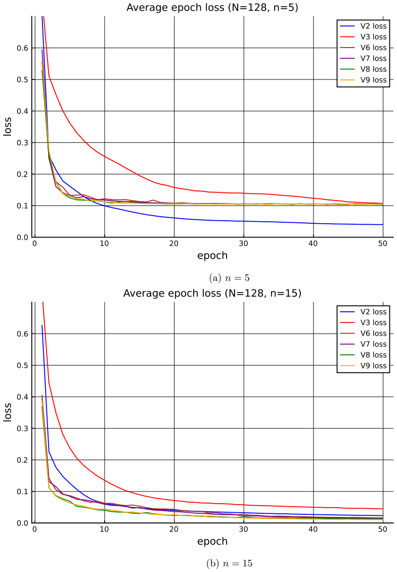
- [Section 4, Tables 13, 16 and 17] Every numerical comparison in the thesis is based on a single training run per variant, with random initialization and random batch draws. The observed differences between variants (e.g., V6-V9 better than V3 on average, V8/V9 slightly ahead of V6/V7, or the comparison to PSD) are therefore not distinguishable from seed-to-seed noise. This matters for the central 'often more accurate' claim: at least three to five seeds with mean and range (or individual points) should be reported for the key comparisons on each example, or the accuracy claims should be explicitly labeled as single-run observations. This also applies to the loss curves in Figures 16, 17, 22 and 26.
- [Section 4.1, Table 10 and Section 3.3.3] The speed test measures only a single PSDLayer manifold update step with a synthetic update vector. The thesis itself notes (end of Section 3.3.3) that each GradientLayer with upscaling factor L = 5N costs O(N^2) per Adam iteration, so the per-iteration cost of the full network remains O(N^2)-dominated; the StiefelAdam speed-up in Table 10 therefore does not by itself establish cheaper end-to-end training. The abstract's claim of 'computational efficiency of the presented learning algorithms' is broader than the evidence presented. Please either report wall-clock training time per epoch (or per iteration) for the full network for the compared variants, or explicitly scope the efficiency claim to the PSDLayer update step (and correspondingly adjust the conclusion).
- [Section 4.2.4, Run 13, Figures 18-19 and Table 14] In the N=256 wave-equation run, the V9 autoencoder 'can keep up' with PSD only for n=10,...,16, loses to PSD for n=17,...,20, shows exploding reduction errors for some (n, mu), and the ROM integration time is roughly 20-25 times that of PSD at the largest reduced dimensions. These results are reported honestly, but they are not a minor caveat: model reduction is most relevant at high dimension, so this is a direct limitation on the abstract's statement that the experiments 'demonstrate the improved accuracy' of the presented algorithms. The accuracy claim should be restated with the observed domain of validity (N=128 across the tested n, and N=256 only for n <= 16), and the failure mode at large n should be discussed (e.g., a hypothesis, or at least a statement of which of the two issues observed in Figure 16 - the initial fast decrease and the subsequent instability - is at play here).
minor comments (5)
- [Appendix A, Figures 13-27] Many appendix plot labels contain corrupted characters or missing letters ('reduced dimensi n n', 'err r', 'Reducti n err rs', '/uni03BC' in axis titles, and 'Vμ' in place of 'V3'); the figures should be regenerated with correct fonts and complete labels.
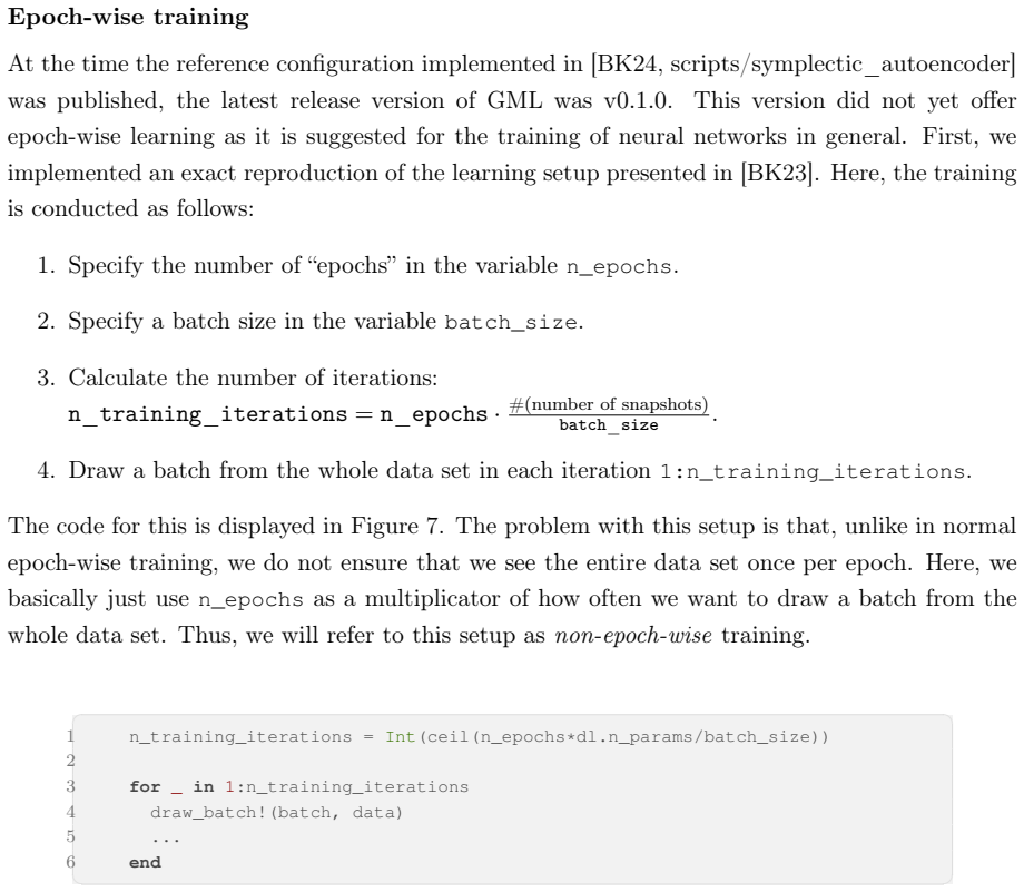
- [Section 3.3.4, Figure 7] The text states n_training_iterations = n_epochs * (#snapshots)/batch_size, but the shown code uses dl.n_params in that formula; if n_params is the number of network parameters rather than the number of snapshots, the non-epoch-wise reproduction does not implement the stated iteration rule and this should be clarified.
- [Section 4.3.4] The phrase 'the (discretized) FOM solution for nu = 0 is constant (int)' appears to mean 'constant in time'; as printed, the parenthetical is not meaningful and should be corrected.
- [References] Reference [Hal00] is cited as an arXiv preprint; the published version (B. Hall, Lie Groups, Lie Algebras, and Representations, Springer GTM 222, 2003) would be more appropriate for a journal version.
- [Section 3.2.3] To position the claimed novelty, the thesis should briefly contrast StiefelAdam with other Riemannian adaptive optimizers in the literature beyond [Bra23] (e.g., Riemannian Adam variants for the Stiefel manifold), even if the comparison is only a remark.
Circularity Check
No significant circularity: the StiefelAdam optimizer is evaluated against external PSD and homogeneous-Adam baselines, and no claimed prediction reduces to its own inputs.
full rationale
The thesis's central contribution is the StiefelAdam update in Algorithm 7 and the direct-on-Stiefel update in Algorithm 8. This optimizer is defined as a modified Adams step on tangent spaces with a transported first-moment cache and a pseudo second-moment cache; it is not derived from, nor fitted to, the accuracy results reported later. The accuracy comparisons (variants V1–V10 versus PSD and versus homogeneous-space Adam) use independent reduction and projection errors on wave and sine-Gordon systems; the speed comparison is backed by explicit per-step operation counts (O(N n^2) versus O(N^2(N-n)+N n^2)) and by the timing experiments in Table 10. The acknowledged divergence of V5 and the subsequently added decay rate eta <- eta * 0.9995 are presented as empirical observations and hyperparameter selection, not as a predicted quantity forced by construction; this is a tuning limitation, not circularity. No parameter is fitted to a subset of data and then reported as a prediction of closely related data. The cited prior work ([BK23], [Bra23], [AMS08]) supplies the network architecture, homogeneous-space retraction, and manifold optimization tools with stated proofs or reproducible implementations; none of these citations is by the present author, and none is used to forbid alternative approaches. Thus no specific reduction of a claimed result to its own inputs can be exhibited, and the paper receives a circularity score of 0.
Assumptions & free parameters
free parameters (3)
- Learning-rate decay in StiefelAdamWithDecay =
eta <- eta * 0.9995 per iteration
- ADAM hyperparameters eta, beta1, beta2, delta =
0.001, 0.9, 0.99, 1e-8
- Network and training hyperparameters =
batch size 32, L=5N, 50 or 100 epochs, 20 training parameter values, 200 time steps
assumptions (5)
- domain assumption The symplectic inverse formula for the decoder and the vanishing symplectic residual justify restricting to symplectic encoder-decoder pairs.
- domain assumption Optimizing only over block-diagonal matrices diag(X, X) with X in St(n, N) is a sufficient restriction of the symplectic Stiefel manifold.
- ad hoc to paper The pseudo second-moment update in Algorithm 7 gives a valid descent direction on the Stiefel manifold.
- ad hoc to paper Transporting only the first-moment cache preserves enough gradient history for Adam-like behavior.
- domain assumption Normalized snapshots together with a reference-state ROM improve training and reconstruction.
invented entities (1)
-
Pseudo second-moment cache B2 in StiefelAdam
Cite this review
Pith. "Pith review of Structure-preserving model reduction of Hamiltonian systems by learning a symplectic autoencoder." pith.science (2026). https://pith.science/paper/UNTVIXI4
@misc{pith2026241113906,
  author       = {Pith},
  title        = {Pith review of: Structure-preserving model reduction of Hamiltonian systems by learning a symplectic autoencoder},
  year         = {2026},
  howpublished = {\url{https://pith.science/paper/UNTVIXI4}},
  note         = {Machine review of arXiv:2411.13906}
}
read the original abstract
Evolutionary partial differential equations play a crucial role in many areas of science and engineering. Spatial discretization of these equations leads to a system of ordinary differential equations which can then be solved by numerical time integration. Such a system is often of very high dimension, making the simulation very time consuming. One way to reduce the computational cost is to approximate the large system by a low-dimensional model using a model reduction approach. This master thesis deals with structure-preserving model reduction of Hamiltonian systems by using machine learning techniques. We discuss a nonlinear approach based on the construction of an encoder-decoder pair that minimizes the approximation error and satisfies symplectic constraints to guarantee the preservation of the structure inherent in Hamiltonian systems. More specifically, we study an autoencoder network that learns a symplectic encoder-decoder pair. Symplecticity poses some additional difficulties, as we need to ensure this structure in each network layer. Since these symplectic constraints are described by the (symplectic) Stiefel manifold, we use manifold optimization techniques to ensure the symplecticity of the encoder and decoder. A particular challenge is to adapt the ADAM optimizer to the manifold structure. We present a modified ADAM optimizer that works directly on the Stiefel manifold and compare it to the existing approach based on homogeneous spaces. In addition, we propose several modifications to the network and training setup that significantly improve the performance and accuracy of the autoencoder. Finally, we numerically validate the modified optimizer and different learning configurations on two Hamiltonian systems, the 1D wave equation and the sine-Gordon equation, and demonstrate the improved accuracy and computational efficiency of the presented learning algorithms.
Figures


Figures from the paper (25 more)





Reference graph
Works this paper leans on
-
[1]
8 1.0 err r R educti n err rs f r Ω=(-0.5,0.5), I=(0,1), N=128, /uni03BC=0.47 PSD reducti n err r V1 reducti n err r V2 reducti n err r Vμ reducti n err r V4 reducti n err r (a) µ = 0 .47 2 4 6 8 10 12 14 reduced dimension n 0.0
-
[2]
8 1.0 e o R eduction e o s fo Ω=(-0.5,0.5), I=(0,1), N=128, /uni03BC=0.51 PSD eduction e o V1 eduction e o V2 eduction e o Vμ eduction e o V4 eduction e o (b) µ = 0 .51 2 4 6 8 10 12 14 reduced dimension n 0.0
-
[3]
8 1.0 e o R eduction e o s fo Ω=(-0.5,0.5), I=(0,1), N=128, /uni03BC=0.55 PSD eduction e o V1 eduction e o V2 eduction e o Vμ eduction e o V4 eduction e o (c) µ = 0 .55 2 4 6 8 10 12 14 reduced dimension n 0.0
-
[4]
76 2 4 6 8 10 12 14 reduced dimensi n n 0.0
8 1.0 e o R eduction e o s fo Ω=(-0.5,0.5), I=(0,1), N=128, /uni03BC=0.625 PSD eduction e o V1 eduction e o V2 eduction e o Vμ eduction e o V4 eduction e o (d) µ = 0 .625 Figure 13: 1D linear wave equation reduction errors for variants V1-V4 and the PSD method in dimensions N = 128 and n = 2, 3, ...,15 for 100 epochs test runs. 76 2 4 6 8 10 12 14 reduced...
-
[5]
8 1.0 err r Pr jecti n err rs f r Ω=(-0.5,0.5), I=(0,1), N=128, /uni03BC=0.47 PSD pr jecti n err r V1 pr jecti n err r V2 pr jecti n err r Vμ pr jecti n err r V4 pr jecti n err r (a) µ = 0 .47 2 4 6 8 10 12 14 reduced dimension n 0.0
-
[6]
8 1.0 error Projection errors for Ω=(-0.5,0.5), I=(0,1), N=128, /uni03BC=0.51 PSD rojection error V1 rojection error V2 rojection error Vμ rojection error V4 rojection error (b) µ = 0 .51 2 4 6 8 10 12 14 reduced dimension n 0.0
-
[7]
8 1.0 error Projection errors for Ω=(-0.5,0.5), I=(0,1), N=128, /uni03BC=0.55 PSD rojection error V1 rojection error V2 rojection error Vμ rojection error V4 rojection error (c) µ = 0 .55 2 4 6 8 10 12 14 reduced dimension n 0.0
-
[8]
77 6 8 10 12 14 reduced dime sio 0.0 0.1
8 1.0 error Projection errors for Ω=(-0.5,0.5), I=(0,1), N=128, /uni03BC=0.625 PSD rojection error V1 rojection error V2 rojection error Vμ rojection error V4 rojection error (d) µ = 0 .625 Figure 14: 1D linear wave equation projection errors for variants V1-V4 and the PSD method in dimensions N = 128 and n = 2, 3, ...,15 for 100 epochs test runs. 77 6 8 ...
Show all 26 references
-
[9]
2 0.3 0.4 0.5 error R eductio errors for Ω=(-0.5,0.5), I=(0,1), N=128, /uni03BC=0.4μ PSD reductio error V3 reductio error V6 reductio error Vμ reductio error V8 reductio error V9 reductio error V10 reductio error (a) µ = 0 .47 6 8 10 12 14 reduced dime sio 0.0 0.1
-
[10]
2 0.3 0.4 0.5 error R eductio errors for Ω=(-0.5,0.5), I=(0,1), N=128, /uni03BC=0.51 PSD reductio error V3 reductio error V6 reductio error Vμ reductio error V8 reductio error V9 reductio error V10 reductio error (b) µ = 0 .51 6 8 10 12 14 reduced dime sio 0.0 0.1
-
[11]
2 0.3 0.4 0.5 error R eductio errors for Ω=(-0.5,0.5), I=(0,1), N=128, /uni03BC=0.55 PSD reductio error V3 reductio error V6 reductio error Vμ reductio error V8 reductio error V9 reductio error V10 reductio error (c) µ = 0 .55 6 8 10 12 14 reduced dime sio 0.0 0.1
-
[12]
78 0 25 50 75 100 epoch 0.0
2 0.3 0.4 0.5 error R eductio errors for Ω=(-0.5,0.5), I=(0,1), N=128, /uni03BC=0.625 PSD reductio error V3 reductio error V6 reductio error Vμ reductio error V8 reductio error V9 reductio error V10 reductio error (d) µ = 0 .625 Figure 15: 1D linear wave equation reduction err...
-
[13]
0 10 20 30 40 50 epoch 0.0
8 1.0 loss A verage epoch loss (N=128, n=15) V3 loss V5 loss V6 loss Figure 16: 1D linear wave equation average epoch target function losses for variants V3, V5 and V6 in dimensions N = 128 and n = 15 for 100 epochs test runs. 0 10 20 30 40 50 epoch 0.0
-
[14]
79 10.0 12.5 15.0 17.5 20.0 reduced dimensi n n 0.0
8 1.0 loss A verage epoch loss (N=128, n=15) V3 loss V6 loss V7 loss V8 loss V9 loss V10 loss Figure 17: 1D linear wave equation average epoch target function losses for variants V3 and V6-V10 in dimensions N = 128 and n = 15 for 50 epochs test runs. 79 10.0 12.5 15.0 17.5 20....
-
[15]
8 1.0 err r R educti n err rs f r Ω=(-0.5,0.5), I=(0,1), N=256, /uni03BC=0.47 PSD reducti n err r Vμ reducti n err r (a) µ = 0 .47 10.0 12.5 15.0 17.5 20.0 reduced dimensi n n 0.0
-
[16]
8 1.0 err r R educti n err rs f r Ω=(-0.5,0.5), I=(0,1), N=256, /uni03BC=0.51 PSD reducti n err r Vμ reducti n err r (b) µ = 0 .51 10.0 12.5 15.0 17.5 20.0 reduced dimensi n n 0.0
-
[17]
8 1.0 err r R educti n err rs f r Ω=(-0.5,0.5), I=(0,1), N=256, /uni03BC=0.55 PSD reducti n err r Vμ reducti n err r (c) µ = 0 .55 10.0 12.5 15.0 17.5 20.0 reduced dimensi n n 0.0
-
[18]
80 −0.50 −0.25 0.00 0.25 0.50 ξ 0.0 0.2 0.4 0.6 0.8 1.0 t 0.00 0.25 0.50
8 1.0 err r R educti n err rs f r Ω=(-0.5,0.5), I=(0,1), N=256, /uni03BC=0.625 PSD reducti n err r Vμ reducti n err r (d) µ = 0 .625 Figure 18: Direct comparison of the1D linear wave equation reduction errors for variant V9 and the PSD method in dimensionsN = 256 and n = 10, ....
-
[20]
−0.50 −0.25 0.00 0.25 0.50 ξ 0.0 0.2 0.4 0.6 0.8 1.0 t 0.00 0.25 0.50
75 1.00 (a) µ = 0.51, V9. −0.50 −0.25 0.00 0.25 0.50 ξ 0.0 0.2 0.4 0.6 0.8 1.0 t 0.00 0.25 0.50
-
[22]
−0.50 −0.25 0.00 0.25 0.50 ξ 0.0 0.2 0.4 0.6 0.8 1.0 t 0.00 0.25 0.50
75 1.00 (b) µ = 0.51, PSD. −0.50 −0.25 0.00 0.25 0.50 ξ 0.0 0.2 0.4 0.6 0.8 1.0 t 0.00 0.25 0.50
-
[24]
−0.50 −0.25 0.00 0.25 0.50 ξ 0.0 0.2 0.4 0.6 0.8 1.0 t 0.00 0.25 0.50
75 1.00 (c) µ = 0.625, V9. −0.50 −0.25 0.00 0.25 0.50 ξ 0.0 0.2 0.4 0.6 0.8 1.0 t 0.00 0.25 0.50
-
[25]
75 1.00 Reconstructed sol tion for Ω=(-0.5,0.5), I=(0,1), N=258 0.00
-
[26]
75 1.00 (d) µ = 0.625, PSD. Figure 19: Comparison of the reconstruction of the1D wave equation from the integrated ROM solution in dimension n = 17 to the full dimensionN = 256 using the autoencoder variant V9 (50 epochs) and the PSD method. 81 5.0 7.5 10.0 12.5 15.0 reduced d...
-
[28]
2 0.3 0.4 0.5 0.6 loss A verage epoch loss (N=128, n=15) V2 loss V3 loss V6 loss V7 loss V8 loss V9 loss (b) n = 15 Figure 22: Comparison of1D sine-Gordon equation (single soliton) average epoch target function losses for variants V2, V3 and V6-V9 in dimension N = 128 for 50 e...
-
[29]
2 0.3 0.4 0.5 0.6 loss A verage epoch loss (N=128, n=5) V2 loss V3 loss V6 loss V7 loss V8 loss V9 loss (a) n = 5 0 10 20 30 40 50 epoch 0.0 0.1
-
[30]
2 0.3 0.4 0.5 0.6 loss A verage epoch loss (N=128, n=15) V2 loss V3 loss V6 loss V7 loss V8 loss V9 loss (b) n = 15 Figure 26: Comparison of 1D sine-Gordon equation (soliton-soliton doublets) average epoch target function losses for variants V2, V3 and V6-V9 in dimension N = 1...
Reviewed August 12, 2026 · model on record in the stance chip above.
Discussion (0). Continue with ORCID to comment.