Variational Multiscale Evolve and Filter Strategies for Convection-Dominated Flows

Francesco Ballarin; Maria Strazzullo; Tom\'as Chac\'on Rebollo; Traian Iliescu

REVIEW 4 major objections 5 minor 62 references

Variational Multiscale Evolve and Filter Strategies for Convection-Dominated Flows

T0 review · 4 major / 5 minor · reviewed 2026-08-12 · deepseek-v4-flash

Challenge this review Re-run · record.json Download PDF Read on arXiv ↗ Review JSON

Pith's one-line read By filtering only the small resolved scales and adding them back to the large scales, the new VMS-EFFC method restores vortex shedding that an over-diffusive evolve-filter smoothing removes, in full-order and reduced-order simulations.

desk verdict The FOM algorithm is formally van Cittert deconvolution of order 1, and the 'significantly more accurate' claim outruns the single-δ evidence; the ROM extension and EPFC variant are the real contributions, worth a serious but demanding referee. read the letter →

arxiv 2411.13957 v2 pith:FS6RHRQC submitted 2024-11-21 math.NA cs.NAphysics.flu-dyn

Maria Strazzullo , Francesco Ballarin , Traian Iliescu , Tomás Chacón Rebollo This is my paper · ORCID

classification math.NAcs.NAphysics.flu-dyn MSC 65M6065N3076D05

keywords evolve-filterregularizationvariationalmultiscaledifferentialfilterreduced-ordermodelconvection-dominatedflowNavier-Stokesequationsapproximatedeconvolutionvortexshedding

verification ladder T0 review T1 audit T2 compute T3 formal

The pith

A machine-rendered reading of the paper's core claim, the machinery that carries it, and where it could break.

The reading

The evolve-filter (EF) method is a simple way to stabilize under-resolved convection-dominated flow simulations: evolve the Navier-Stokes equations, then apply a spatial filter to smooth spurious oscillations. When the filter radius is too large, EF becomes overdiffusive and smooths away physically important features such as vortex shedding. This paper proposes fixing that by splitting the evolved velocity into large and small resolved scales, filtering only the small scales, and adding the filtered small scales back to the large scales. The resulting VMS-EFFC and VMS-EPFC algorithms are claimed to be significantly more accurate than standard EF on a flow past a cylinder at Reynolds number 1000, both in the full-order simulation and in reduced-order models built from it. The authors argue that relative pointwise errors are not the right metric for regularized models, and instead use $L^2$ norms, drag and lift coefficients, and qualitative flow patterns to support the claim.

What carries the argument

The load-bearing mechanism is the correction step: the new velocity is $\mathbf{u}^{n+1} = \bar{\mathbf{w}}^{n+1} + \widetilde{\mathbf{w}'}^{\,n+1}$, where $\mathbf{w}^{n+1}$ is the evolved velocity, $\bar{\mathbf{w}}^{n+1}$ is its large-scale part (obtained by a differential filter of radius $\delta_1$ in VMS-EFFC, or by an $L^2$-projection in VMS-EPFC), and $\widetilde{\mathbf{w}'}^{\,n+1}$ is the small-scale difference $\mathbf{w}' = \mathbf{w} - \bar{\mathbf{w}}$ passed through a second differential filter of radius $\delta_2$. With $\delta_1 = \delta_2$, the output equals $D_1(\mathbf{w}) = 2\bar{\mathbf{w}} - \bar{\bar{\mathbf{w}}}$, the first-order van Cittert approximate deconvolution, so the extra filter loop is precisely an approximate deconvolution that restores some of the energy the first filter removed.

What would settle it

Re-run the cylinder flow test at $Re = 1000$ with a filter radius small enough that the standard EF is not overdiffusive, since the paper concedes EF can then be competitive; if VMS-EFFC no longer improves the velocity $L^2$ norm or drag coefficient, the claimed superiority does not extend beyond the overdiffusive regime. Alternatively, treat the pointwise relative error in the paper's own Figure 11 as the decisive metric, which would invert the conclusion, since EF has the lower error there.

Watch

Extended reading notes

Core claim

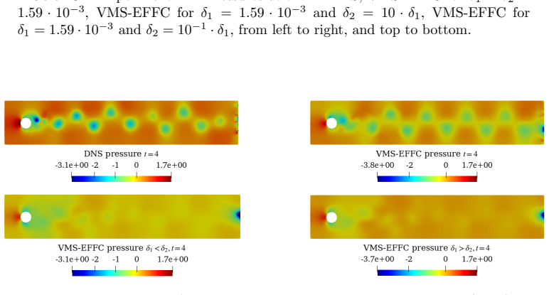
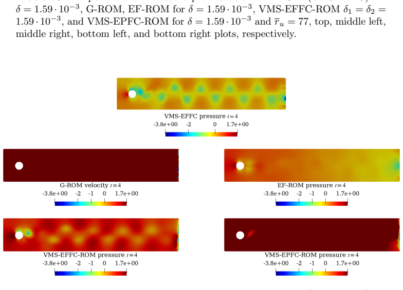
The paper's central discovery is that over-diffusivity in the evolve-filter strategy can be corrected by a scale-separation step: after evolving the velocity, one defines 'large' resolved scales and 'small' resolved scales, applies the differential filter only to the small scales, and forms the new state as the sum of the large scales and the filtered small scales. Two variants are proposed: VMS-EFFC, where the large scales are obtained by a first differential filter, and VMS-EPFC, where a postprocessing $L^2$-projection with grad-div stabilization plays that role. In both variants the filtered small scales serve as a correction that restores features the filter would otherwise destroy. The authors show that when the two filter radii in VMS-EFFC are equal, the algorithm is formally identical to the first-order van Cittert approximate deconvolution operator $D_1(\mathbf{u}) = 2\bar{\mathbf{u}} - \bar{\bar{\mathbf{u}}}$. Numerical tests on flow past a cylinder at $Re = 1000$ indicate that VMS-EFFC is the most accurate strategy among EF, VMS-EPFC, and the ROM variants G-ROM, EF-ROM, VMS-EFFC-ROM, and VMS-EPFC-ROM, based on average quantities and qualitative vortex-shedding behavior.

Load-bearing premise

The paper's accuracy claim depends on rejecting the pointwise relative velocity error, the one metric in which the standard EF has lower error than VMS-EFFC, in favor of average quantities such as $L^2$ norms and qualitative vortex patterns, which the paper judges to be the appropriate measures for regularized models.

Editorial extensions

If this is right

At the FOM level, VMS-EFFC provides a parameter-light way to correct overdiffusive filtering: users keep one filter radius and add a second filter of the same radius plus a sum, instead of tuning a relaxation parameter.
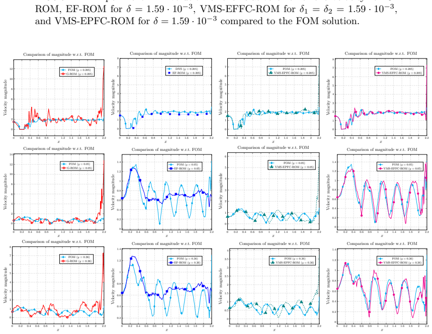
At the ROM level, VMS-EFFC-ROM reduces the average relative velocity error roughly sixfold compared with the Galerkin ROM and threefold compared with VMS-EPFC-ROM, while costing about 115% of the G-ROM CPU time.
The formal identity with the first-order van Cittert operator means the correction is a deconvolution step, aligning VMS-EFFC with a whole family of approximate-deconvolution regularizations.
VMS-EPFC performs worse on pressure and divergence, and the authors recommend VMS-EFFC as the FOM model for ROM construction, so the practical pipeline is VMS-EFFC, POD, VMS-EFFC-ROM.
The lid-driven cavity test at $Re = 7500$ shows the qualitative advantage of VMS-EFFC over EF persists beyond the cylinder benchmark, although the paper notes that relative errors remain high.

Reading between the lines

Editorial extensions of the paper, not claims the author makes directly.

The formal equivalence to $D_1$ suggests a natural extension: replacing the first-order deconvolution by higher-order van Cittert operators $D_n$ could restore even more of the filtered energy; the paper does not test this, but the machinery is in place.
Because the relative-error metric shows EF winning, the practical advantage of VMS-EFFC may lie in statistics and structure rather than pointwise fidelity; applications with phase-sensitive quantities, such as flow control or aeroelastic loads, would need to check whether the phase shift in the lift coefficient matters.
The VMS-EPFC variant's poor pressure reconstruction and divergence levels near $10^{-5}$ hint that the chosen $L^2$-projection is a weak link; a divergence-free or pressure-aware projection could close that gap.
All experiments fix the filter radii at $\delta_1 = \delta_2 = 1.59 \cdot 10^{-3}$, and the paper reports that unequal radii did not help; a systematic sensitivity sweep over $\delta$ at more Reynolds numbers and in three dimensions would directly test whether the correction idea transfers beyond the two benchmarks examined.

Share X Bluesky LinkedIn Reddit HN

Editorial analysis

A structured set of objections, weighed in public.

Desk editor's note, referee report, and a circularity audit.

Desk Editor's Note

read the letter

Two things to know. First, the headline FOM algorithm is not new: VMS-EFFC with equal filter radii is exactly van Cittert approximate deconvolution of order 1, and the authors know it (Remark 4). The novelty that survives is the EPFC variant and the ROM adaptation, neither of which I have seen before in this exact form. Second, the 'significantly more accurate' claim in the abstract is ahead of the evidence: the FOM comparison uses a single deliberately overdiffusive δ, and the one pointwise metric that favors standard EF (relative L2 error, Figure 11) is dismissed as 'not appropriate' without a quantitative justification.

What the paper does well: it is clearly written, modular, and unusually candid. Remark 6 admits the test case is a trade-off and that no method recovers drag, lift, or relative errors. The lid-driven cavity experiment in Remark 9 is a genuine second data point where VMS-EFFC beats EF on both L2 norm and relative error. The ROM section reports computational overhead (115% of G-ROM CPU time), which is the kind of practical detail I trust. The equivalence with AD(1) is stated cleanly instead of being hidden.

Where the soft spots are. The central quantitative claim depends on choosing the L2 norm and qualitative vortex recovery while discarding pointwise relative error. That is not fatal—there are legitimate reasons to prefer average quantities in turbulent flow—but the paper does not provide the standard robustness checks: no δ-sweep, no time-averaged or phase-insensitive error measure, no error bars. The ROM comparison also has a structural bias: the FOM reference and the POD snapshots are all VMS-EFFC, so EF-ROM and G-ROM are tested on data generated by the method they are compared against. That does not invalidate the ROM extension, but it means 'VMS-EFFC-ROM is most accurate' is partly inherited from the FOM choice. Several parameters (γP, ru, δ) are chosen by trial and error, and there is no code.

Overall: a useful, honest numerical study with an overbroad conclusion. The math is straightforward and the algorithms are reproducible from the text. The right response is a serious referee, not a desk reject, but the referee should push for a δ-sweep, a fairer ROM protocol, and a tempered abstract.

Recommendation: send to peer review; require major revisions before acceptance.

Referee Report

4 major / 5 minor

Summary. The paper proposes two filter-based stabilization variants, VMS-EFFC and VMS-EPFC, that modify the standard evolve-filter (EF) strategy by decomposing the evolved velocity into large and small resolved scales, filtering the small scales, and adding the filtered small scales back to the large scales. The authors test these methods on flow past a cylinder at Re = 1000 with a deliberately overdiffusive filter radius, reporting that VMS-EFFC recovers vortex shedding and matches the DNS L2 norm better than EF, while VMS-EPFC is less accurate. They then extend the methods to reduced-order models, proposing VMS-EFFC-ROM and VMS-EPFC-ROM, and report that VMS-EFFC-ROM outperforms G-ROM and EF-ROM in their tests. The paper is primarily a numerical investigation; it includes no convergence analysis or code release.

Significance. If the central claim is established, the paper would offer a simple, modular correction to the overdiffusive behavior of evolve-filter regularization in both FOM and ROM settings, which would be practically useful. The paper is honest about several limitations, including the acknowledged equivalence of VMS-EFFC to van Cittert approximate deconvolution (Remark 4) and the admitted failure of all methods on some metrics. However, the significance is weakened by the fact that the main algorithmic variant is formally identical to a known deconvolution operator, and the numerical evidence is built on a single filter radius and on a metric selection that is justified only qualitatively.

major comments (4)

[Section 5.2, Figs. 8-11; Section 7] The conclusion that VMS-EFFC is 'significantly more accurate' is not supported by a consistent accuracy criterion. The pointwise relative error Eu in Figure 11 favors the standard EF, and the manuscript dismisses this metric as 'not appropriate' without a quantitative justification. At the same time, Remark 6 concedes that parameter changes that reduce the VMS relative errors worsen the average quantities, and Section 5.2 states that none of the methods accurately reproduces CD, CL, or the relative errors. The conclusions in Section 7 even claim improved 'relative errors in time,' which contradicts Figure 11. The authors should either adopt a phase-shift-insensitive error metric (e.g., time-aligned errors, error in dominant Fourier modes, or windowed averages) or explicitly restrict the claim to the specific metrics and parameter regime used.
[Section 5.2, p. 13 and Figs. 4-5] The FOM comparison is conducted at a single, deliberately overdiffusive filter radius, delta = 1.59e-3, chosen 'to showcase the benefits' of the VMS-based filters. The manuscript itself notes that 'for some values of delta, the EF strategy can be as competitive as the VMS-based algorithm,' but it does not quantify this statement. Without a sweep over delta or a well-defined threshold for what constitutes 'too large' a filter radius, the abstract claim that the new algorithms 'yield significantly more accurate results than the standard EF' is not established as a property of the algorithms rather than a property of the selected parameter. A table or plot showing L2 norm and Eu errors for EF and VMS-EFFC across a range of delta values would be the minimal fix.
[Section 6, Algorithms 4-7] The ROM comparison is structurally favorable to VMS-EFFC-ROM because every ROM algorithm (G-ROM, EF-ROM, VMS-EFFC-ROM, VMS-EPFC-ROM) builds its reduced basis from snapshots generated by the VMS-EFFC FOM (step 1 in Algorithms 4-7). With such a basis, the VMS-EFFC-ROM is expected to be closer to the reference FOM solution than a ROM that needs to regularize different dynamics. The claim that VMS-EFFC-ROM outperforms EF-ROM as a regularization strategy therefore requires a fairer test, for example repeating the ROM comparison with snapshots from the EF-FOM (or from the plain NSE FOM) and reporting whether the ranking persists. At minimum, the paper should explicitly state and discuss this construction bias.
[Remark 4, Eq. (4); Section 1] Remark 4 shows that VMS-EFFC with delta1 = delta2 is formally identical to the van Cittert approximate deconvolution operator D1 applied to the evolved velocity. This is an important and candid admission, but it undercuts the paper's novelty claim in the Introduction that this is 'the first time the EF and VMS strategies are combined in correction algorithms.' The VMS-EFFC algorithm is then a known deconvolution operation presented in VMS language, and the ROM extension is closely connected to existing approximate deconvolution ROMs. The authors should reposition the contribution to focus on the VMS interpretation, the EPFC variant, and the ROM formulation, and they should discuss the relation to the approximate deconvolution literature earlier and more prominently.

minor comments (5)

[Table 2, Figure 2, Remark 9] There are several typos: 'Ganeral setting' appears in Table 2 and Figure 2, 'VSM-EFFC' appears in Remark 9, and 'approch' appears in the same remark. These should be corrected.
[Section 5.1] The text refers to 'equation (15)' for the inlet boundary condition in the flow-past-a-cylinder problem, but Eq. (15) is the boundary condition for the lid-driven cavity test in Remark 9. The cross-reference should be to Eq. (12).
[Figure 12 caption] The captions for the center and right panels in the bottom row of Figure 12 are mismatched: the center column is labeled 'VMS-EPFC (y=0.05)' but should be 'VMS-EPFC (y=0.36)', and one of the bottom-right panel labels repeats 'VMS-EPFC (y=0.05)' instead of 'VMS-EFFC (y=0.36)'. This makes the qualitative comparison difficult to follow.
[Algorithm 7, step 7] In Algorithm 7, step 7, the notation shows what appear to be identical quantities on both sides of the assignment for the first set of coefficients, and the index ranges for the zeroed coefficients are written as 'rus + 1, . . . , rus'. The intended truncation of the coefficient vector should be written with distinct symbols (e.g., barred and unbarred coefficients) and with a correct index range.
[General] The paper does not include a data or code availability statement. Given that the conclusions rely entirely on numerical experiments, providing access to the implementation or at least a detailed reproducibility description would strengthen the manuscript.

Circularity Check

1 steps flagged · score 2.0 of 10

Only concrete circular step is the acknowledged equivalence of VMS-EFFC to van Cittert approximate deconvolution; the accuracy comparisons themselves are not circular.

renaming known result [Section 3.1, Remark 4, Eq. (4)]
"We note that the VMS-EFFC velocity, which applies a first differential filter to find u′, a second differential filter to find u′, and then, corrects the large scales, is formally equal to D1(u) since u = u + u′ = u + u − u = 2u − u = D1(u).(4)"

For δ1=δ2, the four-step 'VMS-based' algorithm is, by the paper's own identity, the textbook van Cittert approximate deconvolution operator D1(w)=2w̄−w̄̄. The claimed novelty ('first time the EF and VMS strategies are combined') is therefore a relabeling of a known operator rather than a new construction, and any analysis of VMS-EFFC is automatically an analysis of AD1. The accuracy comparison to EF remains an empirical test of AD1 vs EF, so this renaming does not force the numerical conclusion; hence low severity.

full rationale

The paper's algorithmic definitions are self-contained: EF, VMS-EFFC, and VMS-EPFC are defined by explicit evolve/filter/correct steps, and the FOM accuracy claims are evaluated against an independent DNS on a fine mesh. No parameter is fitted to the DNS error and then reported as a prediction; δ is chosen deliberately large to make EF overdiffusive, and γP is set by a separate numerical study, neither of which is disguised as a derived result. The ROM tests are standard POD reconstructions of the FOM used to generate the snapshots, so the ROM comparison is a consistency check rather than an extrapolation, but it does not reduce any equation to its own output. The one legitimate reduction is Remark 4 / Eq. (4): for δ1=δ2, VMS-EFFC is algebraically identical to the known van Cittert approximate deconvolution operator D1. This undercuts the 'first time' novelty claim but does not vitiate the numerical comparison, which remains a valid empirical comparison of AD1 versus EF. Self-citations such as [51] for grad-div stabilization and consistent filter radii are parameter choices, not load-bearing circular arguments. Overall, the central accuracy claim is not forced by construction, so the circularity score is low.

Assumptions & free parameters 5 free parameters · 5 assumptions · 0 invented entities

The central claim rests on several manually chosen parameters (filter radii, grad-div coefficients, POD truncation, EPFC mode count) and on standard but unproven assumptions about VMS decomposition and filter smoothing. No new physical entities are introduced.

free parameters (5)

filter radius delta = 1.59e-3
Used for EF, VMS-EFFC and VMS-EPFC; chosen to demonstrate overdiffusive EF behavior; no sensitivity sweep for the main comparison.
grad-div parameter gamma_P = 0.01
Used in VMS-EPFC projection; selected by trial and error (Remark 7), tuning results not shown.
number of retained POD modes ru = 140
Retains 99.5% velocity energy; choice affects ROM accuracy.
number of pressure POD modes rp = 15
Retains 99.9% pressure energy; chosen to recover vortex shedding.
EPFC large-scale mode count ru_EPFC = 77
Set to floor(ru/2); other values gave worse results (Remark 10), so this is a tuned hyperparameter.

assumptions (5)

domain assumption Incompressible Navier-Stokes equations with free-flow outlet boundary conditions are the correct model for the test flows.
Used throughout; standard for CFD validation.
domain assumption The discrete velocity and pressure spaces admit a VMS direct-sum decomposition into large and small resolved scales (Eq. 3).
Standard VMS assumption; invoked in Section 3.
standard math The differential filter with homogeneous Neumann boundary conditions is an effective smoothing operator.
Classical filter; relies on elliptic regularity.
domain assumption Taylor-Hood P2-P1 finite elements and Galerkin discretization are adequate for the under-resolved regime with additional regularization.
Standard choice; not justified in the paper beyond literature references.
standard math Supremizer stabilization of the ROM velocity space guarantees inf-sup stability of the reduced problem.
Standard ROM technique; cited from [2,46].

how reviews work

0 comments

Cite this review

Pith. "Pith review of Variational Multiscale Evolve and Filter Strategies for Convection-Dominated Flows." pith.science (2026). https://pith.science/paper/FS6RHRQC

@misc{pith2026241113957,
  author       = {Pith},
  title        = {Pith review of: Variational Multiscale Evolve and Filter Strategies for Convection-Dominated Flows},
  year         = {2026},
  howpublished = {\url{https://pith.science/paper/FS6RHRQC}},
  note         = {Machine review of arXiv:2411.13957}
}

read the original abstract

The evolve-filter (EF) model is a filter-based numerical stabilization for under-resolved convection-dominated flows. EF is a simple, modular, and effective strategy for both full-order models (FOMs) and reduced-order models (ROMs). It is well-known, however, that when the filter radius is too large, EF can be overdiffusive and yield inaccurate results. To alleviate this, EF is usually supplemented with a relaxation step. The relaxation parameter, however, is very sensitive with respect to the model parameters. In this paper, we propose a novel strategy to alleviate the EF overdiffusivity for a large filter radius. Specifically, we leverage the variational multiscale (VMS) framework to separate the large resolved scales from the small resolved scales in the evolved velocity, and we use the filtered small scales to correct the large scales. Furthermore, in the new VMS-EF strategy, we use two different ways to decompose the evolved velocity: the VMS Evolve-Filter-Filter-Correct (VMS-EFFC) and the VMS Evolve-Postprocess-Filter-Correct (VMS-EPFC) algorithms. The new VMS-based algorithms yield significantly more accurate results than the standard EF in both the FOM and the ROM simulations of a flow past a cylinder at Reynolds number Re = 1000.

Figures

Figures reproduced from arXiv: 2411.13957 by the authors.

**Figure 1.** Spatial domain Ω: schematic representation. ΓD = Γin ∪ Γw. Homogeneous Dirichlet conditions are applied on the solid cyan boundary. The inlet boundary Γin is represented by a dotted magenta line. The “free flow” boundary ΓN is depicted by a dashed black line [PITH_FULL_IMAGE:figures/full_fig_p012_1.png] view at source ↗

**Figure 2.** Ganeral setting. Coarse mesh (M1) and fine mesh (M2), left and right plots, respectively [PITH_FULL_IMAGE:figures/full_fig_p013_2.png] view at source ↗

**Figure 3.** General setting. Velocity profiles for NSE-no-filtered simulation on the coarse mesh (M1) at t = 1 and t = 4, left and right plots, respectively. The EF, VMS-EFFC, and VMS-EPFC algorithms are applied on a triangular mesh (left plot in [PITH_FULL_IMAGE:figures/full_fig_p013_3.png] view at source ↗

Figures from the paper (34 more)

**Figure 4.** Figure 4: Experiment 1. Velocity profiles at t = 1: DNS (top left), EF (top right) for δ = 1.59 · 10−3 , VMS-EFFC (bottom left) for δ1 = δ2 = 1.59 · 10−3 , and VMSEPFC (bottom right) for δ = 1.59 · 10−3 [PITH_FULL_IMAGE:figures/full_fig_p014_4.png]

**Figure 5.** Figure 5: Experiment 1. Velocity profiles at t = 4: DNS (top left), EF (top right) for δ = 1.59 · 10−3 , VMS-EFFC (bottom left) for δ1 = δ2 = 1.59 · 10−3 , and VMSEPFC (bottom right) for δ = 1.59 · 10−3 [PITH_FULL_IMAGE:figures/full_fig_p015_5.png]

**Figure 6.** Figure 6: Experiment 1. Vorticity profiles at t = 1: DNS (top left), EF (top right) for δ = 1.59 · 10−3 , VMS-EFFC (bottom left) for δ1 = δ2 = 1.59 · 10−3 , and VMS-EPFC (bottom right) for δ = 1.59 · 10−3 [PITH_FULL_IMAGE:figures/full_fig_p015_6.png]

**Figure 7.** Figure 7: Experiment 1. Vorticity profiles at t = 4: DNS (top left), EF (top right) for δ = 1.59 · 10−3 , VMS-EFFC (bottom left) for δ1 = δ2 = 1.59 · 10−3 , and VMS-EPFC (bottom right) for δ = 1.59 · 10−3 [PITH_FULL_IMAGE:figures/full_fig_p015_7.png]

**Figure 8.** Figure 8: Experiment 1. Left: Velocity L 2 -norms in time for EF with δ = 1.59 · 10−3 , VMS-EFFC for δ1 = δ2 = 1.59 · 10−3 , and VMS-EPFC for δ = 1.59 · 10−3 compared to the DNS solution. Right: divergence evolution for EF with δ = 1.59 · 10−3 , VMS-EFFC with δ1 = δ2 = 1.59 · 10…

**Figure 9.** Figure 9: Experiment 1. CD(t): DNS, EF for δ = 1.59 · 10−3 , VMS-EFFC for δ1 = δ2 = 1.59 · 10−3 , and VMS-EPFC for δ = 1.59 · 10−3 , left plot. In the right plot, we show the same quantities but we exclude the VMS-EPFC from the results [PITH_FULL_IMAGE:figures/full_fig_p016_9.png]

**Figure 10.** Figure 10: Experiment 1. CL(t): DNS, EF for δ = 1.59 · 10−3 , VMS-EFFC for δ1 = δ2 = 1.59 · 10−3 , and VMS-EPFC for δ = 1.59 · 10−3 , left plot. In the right plot, we show the same quantities but we exclude the VMS-EPFC from the results. In Figures 9 and 10, we show the drag and…

**Figure 11.** Figure 11: Experiment 1. Velocity relative error in time for EF with δ = 1.59 · 10−3 , VMS-EFFC for δ1 = δ2 = 1.59 · 10−3 , and VMS-EPFC for δ = 1.59 · 10−3 compared to the DNS solution. In conclusion, due to the poor EF and VMS-EPFC performances, we choose VMS-EFFC as the FOM m…

**Figure 12.** Figure 12: Experiment 1. Comparison of the velocity for fixed y values and varying x values. DNS results are shown for comparison purposes. Top row: EF for δ = 1.59·10−3 (left), VMS-EPFC for δ1 = δ2 = 1.59·10−3 (center), and VMS-EFFC for δ = 1.59 · 10−3 (right) for y = 0.205. C…

**Figure 13.** Figure 13: Experiment 1. Velocity profiles for EFR simulation on the coarse mesh (M1) for t = 1 and t = 4, left and right plots, respectively. Remark 9 (Robustness of the VMS-EFFC approch). To test the robustness of the VMS-EFFC approach, i.e., the best approach for the flow pas…

**Figure 14.** Figure 14: Experiment 1 (lid-driven cavity). Velocity profiles at t = 1: DNS (left), EF (center) for δ = 1.59 · 10−3 , and VMS-EFFC (right) for δ1 = δ2 = 1.59 · 10−3 [PITH_FULL_IMAGE:figures/full_fig_p021_14.png]

**Figure 15.** Figure 15: Experiment 1 (lid-driven cavity). Velocity profiles at t = 2: DNS (left), EF (center) for δ = 1.59 · 10−3 , and VMS-EFFC (right) for δ1 = δ2 = 1.59 · 10−3 [PITH_FULL_IMAGE:figures/full_fig_p021_15.png]

**Figure 16.** Figure 16: Experiment 1 (lid-driven cavity). Left: Velocity L 2 -norms in time for DNS, EF for δ = 1.59 · 10−3 , and VMS-EFFC for δ1 = δ2 = 1.59 · 10−3 . Right: Velocity relative error in time for DNS, EF for δ = 1.59 · 10−3 , and VMS-EFFC for δ1 = δ2 = 1.59 · 10−3 . 6. ROM Resu…

**Figure 17.** Figure 17: Experiment 2. Velocity profiles at t = 1: FOM (VMS-EFFC) for δ = 1.59 · 10−3 , G-ROM, EF-ROM for δ = 1.59 · 10−3 , VMS-EFFC-ROM for δ1 = δ2 = 1.59 · 10−3 , VMS-EPFC-ROM for δ = 1.59 · 10−3 and ru = 77, top, middle left, middle right, bottom left, and bottom right plot…

**Figure 18.** Figure 18: Experiment 2. Velocity profiles at t = 4: FOM (VMS-EFFC) for δ = 1.59 · 10−3 , G-ROM, EF-ROM for δ = 1.59 · 10−3 , VMS-EFFC-ROM for δ1 = δ2 = 1.59 · 10−3 , VMS-EPFC-ROM for δ = 1.59 · 10−3 and ru = 77, top, middle left, middle right, bottom left, and bottom right plot…

**Figure 19.** Figure 19: Experiment 2. Left: Evolution of the squared L 2 -norms of the velocity for G-ROM, EF-ROM for δ = 1.59 · 10−3 , VMS-EFFC for δ1 = δ2 = 1.59 · 10−3 , and VMS-EPFC for δ = 1.59 · 10−3 and ru = 77 compared to the FOM solution (VMS-EFFC) for δ = 1.59 · 10−3 . The left plo…

**Figure 20.** Figure 20: Experiment 2. CD(t): FOM (VMS-EFFC), for δ = 1.59 · 10−3 , EFROM, VMS-EFFC-ROM for δ1 = δ2 = 1.59 · 10−3 , and VMS-EPFC-ROM for δ = 1.59 · 10−3 and ru = 77. The left plot shows G-ROM, which is omitted in the right plot for clarity. To better understand the error beha…

**Figure 21.** Figure 21: Experiment 2. CL(t): FOM (VMS-EFFC), for δ = 1.59 · 10−3 , EFROM, VMS-EFFC-ROM for δ1 = δ2 = 1.59 · 10−3 , and VMS-EPFC-ROM for δ = 1.59 · 10−3 and ru = 77. The left plot shows G-ROM, which is omitted in the right plot for clarity [PITH_FULL_IMAGE:figures/full_fig_p…

**Figure 22.** Figure 22: Experiment 2. Evolution of the relative error of the velocity for GROM, EF-ROM for δ = 1.59 · 10−3 , VMS-EFFC-ROM for δ1 = δ2 = 1.59 · 10−3 , and VMS-EPFC-ROM for δ = 1.59 · 10−3 compared to the FOM solution. 0 0.2 0.4 0.6 0.8 1 1.2 1.4 1.6 1.8 2 2.2 0 2 4 6 8 10 12 …

**Figure 23.** Figure 23: Experiment 2. Comparison of the ROM velocity magnitude with the FOM velocity magnitude for varying x and fixed y. Top row from left to right: GROM, EF-ROM for δ = 1.59·10−3 , VMS-EPFC-ROM for δ1 = δ2 = 1.59·10−3 , and VMS-EFFC-ROM for δ = 1.59·10−3 for y = 0.205. Cen…

**Figure 24.** Figure 24: Experiment A1. Velocity profiles at t = 1: DNS, VMS-EFFC for δ1 = δ2 = 1.59 · 10−3 , VMS-EFFC for δ1 = 1.59 · 10−3 and δ2 = 10 · δ1, and VMSEFFC for δ1 = 1.59 · 10−3 and δ2 = 10−1 δ1, top left and right, bottom left, and right plots, respectively. In this numerical s…

**Figure 27.** Figure 27: The use of δ1 < δ2 damps out the oscillations of the drag and lift coefficients [PITH_FULL_IMAGE:figures/full_fig_p031_27.png]

**Figure 25.** Figure 25: Experiment A1. Velocity profiles at t = 4: DNS, VMS-EFFC for δ1 = δ2 = 1.59 · 10−3 , VMS-EFFC for δ1 = 1.59 · 10−3 and δ2 = 10 · δ1, and VMSEFFC for δ1 = 1.59 · 10−3 and δ2 = 10−1 δ1, top left and right, bottom left, and right plots, respectively. 0 0.5 1 1.5 2 2.5 3…

**Figure 26.** Figure 26: Experiment A1. Evolution of the L 2 -norms of the velocity for DNS for δ = 1.59·10−3 , VMS-EFFC for δ = 1.59·10−3 and δ2 = 1.59·10−2 , and VMS-EFFC for δ = 1.59 · 10−3 and δ2 = 1.59 · 10−4 . Using δ1 > δ2, helps to recover the magnitude of the drag and lift coefficien…

**Figure 27.** Figure 27: Experiment 1. CD(t) and CL(t) in time for DNS for δ = 1.59 · 10−3 , VMS-EFFC for δ = 1.59 · 10−3 and δ2 = 1.59 · 10−2 , and VMS-EFFC for δ = 1.59 · 10−3 and δ2 = 1.59 · 10−4 , left and right plots, respectively. Appendix B. Additional FOM Results: Pressure This append…

**Figure 28.** Figure 28: Experiment 1. Pressure profiles at t = 1: DNS, EF for δ = 1.59 · 10−3 , VMS-EFFC for δ1 = δ2 = 1.59 · 10−3 , and VMS-EPFC for δ = 1.59 · 10−3 and ru = 15, from left to right, and top to bottom [PITH_FULL_IMAGE:figures/full_fig_p033_28.png]

**Figure 29.** Figure 29: Experiment 1. Pressure profiles at t = 4: DNS, EF for δ = 1.59 · 10−3 , VMS-EFFC for δ1 = δ2 = 1.59 · 10−3 , and VMS-EPFC for δ = 1.59 · 10−3 , from left to right, and top to bottom. 0 0.5 1 1.5 2 2.5 3 3.5 4 10−2 10−1 100 101 102 103 104 105 106 107 t L 2-norm Compar…

**Figure 30.** Figure 30: Experiment 1. Evolution of the L 2 -norms of the pressure for DNS, EF for δ = 1.59 · 10−3 , VMS-EFFC for δ1 = δ2 = 1.59 · 10−3 , and VMS-EPFC for δ = 1.59 · 10−3 . The results are consistent with the behavior of the velocity fields in the respective experiments. In wh…

**Figure 31.** Figure 31: Experiment A1. Pressures at t = 1: DNS, VMS-EFFC for δ1 = δ2 = 1.59 · 10−3 , VMS-EFFC for δ1 = 1.59 · 10−3 and δ2 = 10 · δ1, VMS-EFFC for δ1 = 1.59 · 10−3 and δ2 = 10−1 · δ1, from left to right, and top to bottom [PITH_FULL_IMAGE:figures/full_fig_p035_31.png]

**Figure 32.** Figure 32: Experiment A1. Pressures at t = 4: DNS, VMS-EFFC for δ1 = δ2 = 1.59 · 10−3 , VMS-EFFC for δ1 = 1.59 · 10−3 and δ2 = 10 · δ1, VMS-EFFC for δ1 = 1.59 · 10−3 and δ2 = 10−1 · δ1, from left to right, and top to bottom. 0 0.5 1 1.5 2 2.5 3 3.5 4 10−1 100 101 t L 2-norm Comp…

**Figure 33.** Figure 33: Experiment A1. Evolution of the squared L 2 -norms of the pressure DNS, EF for δ = 1.59 · 10−3 , VMS-EFFC for δ = 1.59 · 10−3 and δ2 = 1.59 · 10−2 , and VMS-EFFC for δ = 1.59 · 10−3 and δ2 = 1.59 · 10−4 , left and right plots, respectively [PITH_FULL_IMAGE:figures/fu…

**Figure 34.** Figure 34: Experiment 2. Pressure profiles at t = 1: FOM (VMS-EFFC) for δ = 1.59 · 10−3 , G-ROM, EF-ROM for δ = 1.59 · 10−3 , VMS-EFFC-ROM δ1 = δ2 = 1.59 · 10−3 , and VMS-EPFC-ROM for δ = 1.59 · 10−3 and ru = 77, top, middle left, middle right, bottom left, and bottom right plot…

**Figure 35.** Figure 35: Experiment 2. Pressure profiles at t = 4: FOM (VMS-EFFC) for δ = 1.59 · 10−3 , G-ROM, EF-ROM for δ = 1.59 · 10−3 , VMS-EFFC-ROM δ1 = δ2 = 1.59 · 10−3 , and VMS-EPFC-ROM for δ = 1.59 · 10−3 and ru = 77, top, middle left, middle right, bottom left, and bottom right plot…

**Figure 36.** Figure 36: Experiment 2. Left and right: Evolution of the squared L 2 -norms of the pressure for G-ROM, EF-ROM for δ = 1.59 · 10−3 , VMS-EFFC for δ1 = δ2 = 1.59 · 10−3 , VMS-EPFC for δ = 1.59 · 10−3 and ru = 77, and the FOM solution (VMS-EFFC) for δ = 1.59 · 10−3 . The left plot…

Discussion (0). Continue with ORCID to comment.

Reference graph

Works this paper leans on

62 extracted references · 41 canonical work pages

[1]

Aza ¨ ıez, T

M. Aza ¨ ıez, T. Chac´ on Rebollo, M. Oulghelou, and I. S´ anchez Mu˜ noz. Least-squares pressure recovery in reduced order methods for incompressible flows. J. Comput. Phys. , 519:113397, 2024. doi:10.1016/j.jcp.2024.113397

arXiv 2024
[2]

Ballarin, A

F. Ballarin, A. Manzoni, A. Quarteroni, and G. Rozza. Supremizer stabilization of POD–Galerkin approximation of parametrized steady incompressible Navier–Stokes equations. Int. J. Numer. Meth. Engng. , 102:1136–1161,

work page
[3]

Barrault, Y

M. Barrault, Y. Maday, N. C. Nguyen, and A. T. Patera. An ‘empirical interpolation’ method: Application to efficient reduced-basis discretization of partial differential equations. C. R. Acad. Sci. Paris, Ser. I , 339:667–672,

work page
[4]

Benner, M

P. Benner, M. Ohlberger, A. Cohen, and K. Willcox. Model Reduction and Approximation: Theory and Algo- rithms. SIAM, 2017

work page 2017
[5]

L. C. Berselli, T. Iliescu, and W. J. Layton. Mathematics of Large Eddy Simulation of Turbulent Flows . Scientific Computation. Springer-Verlag, Berlin, 2006

work page 2006
[6]

Bertagna, A

L. Bertagna, A. Quaini, and A. Veneziani. Deconvolution-based nonlinear filtering for incompressible flows at moderately large Reynolds numbers. Int. J. Num. Meth. Fluids , 81(8):463–488, 2016. doi:10.1002/fld.4192

work page doi:10.1002/fld.4192 2016
[7]

J. P. Boyd. Two comments on filtering (artificial viscosity) for Chebyshev and Legendre spectral and spectral element methods: preserving boundary conditions and interpretation of the filter as a diffusion. J. Comput. Phys., 143(1):283–288, 1998. doi:10.1006/jcph.1998.5961

arXiv 1998
[8]

J. P. Boyd. Chebyshev and Fourier Spectral Methods . Dover Publications, 2001

work page 2001

Show all 62 references

[9]

Burkardt, M

J. Burkardt, M. Gunzburger, and H. Lee. POD and CVT-based reduced-order modeling of Navier–Stokes flows. Comput. Methods Appl. Mech. Engrg. , 196(1-3):337–355, 2006. doi:10.1016/j.cma.2006.04.004

2006 doi
[10]

Canuto, M

C. Canuto, M. Y. Hussaini, A. Quarteroni, and T. A. Zang. Spectral Methods in Fluid Dynamics. Springer Series in Computational Physics. Springer-Verlag, New York, 1988

1988
[11]

DeCaria, W

V. DeCaria, W. Layton, A. Pakzad, Y. Rong, N. Sahin, and H. Zhao. On the determination of the grad-div criterion. J. Math. Anal. Appl. , 467(2):1032–1037, 2018. doi:10.1016/j.jmaa.2018.07.040

2018 doi
[12]

F. G. Eroglu, S. Kaya, and L. G. Rebholz. A modular regularized variational multiscale proper orthogonal decomposition for incompressible flows. Comput. Methods Appl. Mech. Eng. , 325:350–368, 2017. doi:10.1016/ j.cma.2017.07.017

2017
[13]

V. J. Ervin, W. J. Layton, and M. Neda. Numerical analysis of filter-based stabilization for evolution equations. SIAM J. Numer. Anal. , 50(5):2307–2335, 2012. doi:10.1137/100782048

2012 doi
[14]

P. F. Fischer and J. Mullen. Filter-based stabilization of spectral element methods. C. R. Acad. Sci. Paris S´ er. I Math. , 332(3):265–270, 2001. doi:10.1016/S0764-4442(00)01763-8

2001 doi
[15]

M. Germano. Differential filters for the large eddy numerical simulation of turbulent flows. Phys. Fluids , 29(6):1755–1757, 1986. doi:10.1063/1.865649

1986 doi
[16]

M. Germano. Differential filters of elliptic type. Phys. Fluids , 29(6):1757–1758, 1986. doi:10.1063/1.865650

1986 doi
[17]

Girfoglio, A

M. Girfoglio, A. Quaini, and G. Rozza. A finite volume approximation of the Navier-Stokes equations with nonlinear filtering stabilization. Comput. Fluids , 187:27–45, 2019. doi:10.1016/j.compfluid.2019.05.001

2019 doi
[18]

Girfoglio, A

M. Girfoglio, A. Quaini, and G. Rozza. A POD-Galerkin reduced order model for a LES filtering approach. J. Comput. Phys. , 436:110260, 2021. doi:10.1016/j.jcp.2021.110260

2021
[19]

J. S. Hesthaven, G. Rozza, and B. Stamm. Certified Reduced Basis Methods for Parametrized Partial Differential Equations. Springer, 2015

2015
[20]

T. J. Hughes and J. R. Stewart. A space-time formulation for multiscale phenomena. J. Comput. Appl. Math. , 74(1-2):217–229, 1996. doi:10.1016/0377-0427(96)00025-8

1996 doi
[21]

T. J. R. Hughes, G. R. Feij´ oo, L. Mazzei, and J.-B. Quincy. The variational multiscale method – a para- digm for computational mechanics. Comput. Methods Appl. Mech. Engrg. , 166(1):3–24, 1998. doi:10.1016/ S0045-7825(98)00079-6

1998
[22]

Iliescu and Z

T. Iliescu and Z. Wang. Variational multiscale proper orthogonal decomposition: Convection- dominated convection-diffusion-reaction equations. Math. Comput. , 82(283):1357–1378, 2013. doi: 10.1090/S0025-5718-2013-02683-X

2013 doi
[23]

Iliescu and Z

T. Iliescu and Z. Wang. Variational multiscale proper orthogonal decomposition: Navier-Stokes equations. Num. Meth. P.D.E.s , 30(2):641–663, 2014. doi:10.1002/num.21835

2014 doi
[24]

V. John, A. Linke, C. Merdon, M. Neilan, and L. G. Rebholz. On the divergence constraint in mixed finite element methods for incompressible flows. SIAM Rev., 59(3):492–544, 2017. doi:10.1137/15M1047696

2017 doi
[25]

Kaneko, P.-H

K. Kaneko, P.-H. Tsai, and P. Fischer. Towards model order reduction for fluid-thermal analysis. Nucl. Eng. Des., 370:110866, 2020. doi:10.1016/j.nucengdes.2020.110866

2020
[26]

B. Koc, S. Rubino, T. C. Rebollo, and T. Iliescu. Residual data-driven variational multiscale reduced order models for parameter dependent problems, 2023. arXiv:2208.00059. 30 M. STRAZZULLO, F. BALLARIN, T. ILIESCU, T. CHAC ´ON REBOLLO

2023 arXiv
[27]

Layton, C

W. Layton, C. C. Manica, M. Neda, M. Olshanskii, and L. G. Rebholz. On the accuracy of the rotation form in simulations of the Navier–Stokes equations. J. Comput. Phys. , 228(9):3433–3447, 2009. doi:10.1016/j.jcp. 2009.01.027

2009 doi
[28]

Layton, C

W. Layton, C. C. Manica, M. Neda, and L. G. Rebholz. Numerical analysis and computational testing of a high accuracy Leray-deconvolution model of turbulence. Num. Meth. P.D.E.s, 24(2):555–582, 2008. doi:10.1002/num. 20281

2008 doi
[29]

Layton, N

W. Layton, N. Mays, M. Neda, and C. Trenchea. Numerical analysis of modular regularization methods for the BDF2 time discretization of the Navier-Stokes equations. ESAIM: Math. Model. Numer. Anal. , 48(3):765–793,
[30]

Layton, L

W. Layton, L. R¨ ohe, and H. Tran. Explicitly uncoupled VMS stabilization of fluid flow. Comput. Methods Appl. Mech. Eng., 200(45):3183–3199, 2011. doi:10.1016/j.cma.2011.06.015

2011 doi
[31]

W. J. Layton. Introduction to the Numerical Analysis of Incompressible Viscous Flows , volume 6. Society for Industrial and Applied Mathematics (SIAM), 2008

2008
[32]

W. J. Layton and L. G. Rebholz. Approximate Deconvolution Models of Turbulence: Analysis, Phenomenology and Numerical Analysis , volume 2042. Springer Berlin Heidelberg, 2012

2012
[33]

A. Logg, K. Mardal, and G. Wells. Automated Solution of Differential Equations by the Finite Element Method . Springer-Verlag, Berlin, 2012

2012
[34]

C. Mou, E. Merzari, O. San, and T. Iliescu. An energy-based lengthscale for reduced order models of turbulent flows. Nucl. Eng. Des. , 412:112454, 2023. doi:10.1016/j.nucengdes.2023.112454

2023
[35]

J. S. Mullen and P. F. Fischer. Filtering techniques for complex geometry fluid flows. Commun. Numer. Meth. Engng., 15(1):9–18, 1999. doi:10.1002/(SICI)1099-0887(199901)15:1<9::AID-CNM219>3.0.CO;2-Y

1999 doi
[36]

B. R. Noack, M. Morzynski, and G. Tadmor. Reduced-Order Modelling for Flow Control , volume 528. Springer Verlag, 2011

2011
[37]

Pacciarini and G

P. Pacciarini and G. Rozza. Stabilized reduced basis method for parametrized advection–diffusion PDEs.Comput. Meth. Appl. Mech. Eng. , 274:1–18, 2014. doi:10.1016/j.cma.2014.02.005

2014 doi
[38]

Filter-based stabilization of spectral element methods

R. Pasquetti and C. J. Xu. Comments on “Filter-based stabilization of spectral element methods”. J. Comput. Phys., 182(2):646–650, 2002. doi:10.1006/jcph.2002.7178

2002
[39]

Prud’Homme, D

C. Prud’Homme, D. V. Rovas, K. Veroy, L. Machiels, Y. Maday, A. Patera, and G. Turinici. Reliable real-time solution of parametrized partial differential equations: Reduced-basis output bound methods. J. Fluids Eng. , 124(1):70–80, 2002. doi:10.1115/1.1448332

2002 doi
[40]

Quarteroni

A. Quarteroni. Numerical Models for Differential Problems , volume 2. Springer, 2014

2014
[41]

Quarteroni, A

A. Quarteroni, A. Manzoni, and F. Negri. Reduced Basis Methods for Partial Differential Equations: An Intro- duction, volume 92. Springer, 2015

2015
[42]

T. C. Rebollo and R. Lewandowski. Mathematical and Numerical Foundations of Turbulence Models and Appli- cations. Springer, 2014

2014
[43]

H. G. Roos, M. Stynes, and L. Tobiska. Robust Numerical Methods for Singularly Perturbed Differential Equa- tions: Convection-Diffusion-Reaction and Flow Problems., volume 24 of Springer Series in Computational Math- ematics. Springer, second edition, 2008

2008
[44]

Rozza, F

G. Rozza, F. Ballarin, L. Scandurra, and F. Pichi. Real Time Reduced Order Computational Mechanics . SISSA Springer Series. Springer Cham, 2024

2024
[45]

Rozza, D

G. Rozza, D. Huynh, and A. Patera. Reduced basis approximation and a posteriori error estimation for affinely parametrized elliptic coercive partial differential equations: Application to transport and continuum mechanics. Arch. Comput. Methods Eng. , 15(3):229–275, 2008. doi:...

2008 doi
[46]

Rozza and K

G. Rozza and K. Veroy. On the stability of the reduced basis method for Stokes equations in parametrized domains. Comput. Methods Appl. Mech. Engrg. , 196(7):1244–1260, 2007. doi:10.1016/j.cma.2006.09.005

2007 doi
[47]

Sabetghadam and A

F. Sabetghadam and A. Jafarpour. α regularization of the POD-Galerkin dynamical systems of the Kuramoto– Sivashinsky equation. Appl. Math. Comput. , 218(10):6012–6026, 2012. doi:10.1016/j.amc.2011.11.083

2012 doi
[48]

P. Sagaut. Large Eddy Simulation for Incompressible Flows . Scientific Computation. Springer-Verlag, Berlin, third edition, 2006

2006
[49]

Sanfilippo, I

A. Sanfilippo, I. Moore, F. Ballarin, and T. Iliescu. Approximate deconvolution leray reduced order model for convection-dominated flows. Finite Elem. Anal. Des. , 226, 2023. doi:10.1016/j.finel.2023.104021

2023
[50]

Stabile, F

G. Stabile, F. Ballarin, G. Zuccarino, and G. Rozza. A reduced order variational multiscale approach for turbulent flows. Adv. Comput. Math. , pages 1–20, 2019. doi:10.1007/s10444-019-09712-x

2019 doi
[51]

Strazzullo, M

M. Strazzullo, M. Girfoglio, F. Ballarin, T. Iliescu, and G. Rozza. Consistency of the full and reduced order models for evolve-filter-relax regularization of convection-dominated, marginally-resolved flows.International Journal for Numerical Methods in Engineering , 123(14):3...

2022 doi
[52]

R. Temam. Navier-Stokes equations: Theory and numerical analysis , volume 2. American Mathematical Society, 2001

2001
[53]

Van Reeuwijk, H

M. Van Reeuwijk, H. Jonker, and K. Hanjali´ c. Incompressibility of the Leray- α model for wall-bounded flows. Phys. Fluids , 18(1):018103, 2006. doi:10.1063/1.2166459

2006 doi
[54]

Z. Wang, I. Akhtar, J. Borggaard, and T. Iliescu. Two-level discretizations of nonlinear closure models for proper orthogonal decomposition. J. Comput. Phys. , 230:126–146, 2011. doi:10.1016/j.jcp.2010.09.015. FOM AND ROM VMS-BASED EF STRATEGIES 31

2011 doi
[55]

Z. Wang, I. Akhtar, J. Borggaard, and T. Iliescu. Proper orthogonal decomposition closure models for turbulent flows: A numerical comparison. Comput. Meth. Appl. Mech. Eng. , 237-240:10–26, 2012. doi:10.1016/j.cma. 2012.04.015

2012 doi
[56]

Wells, Z

D. Wells, Z. Wang, X. Xie, and T. Iliescu. An evolve-then-filter regularized reduced order model for convection- dominated flows. Int. J. Num. Meth. Fluids , 84:598––615, 2017. doi:10.1002/fld.4363

2017 doi
[57]

Zoccolan, M

F. Zoccolan, M. Strazzullo, and G. Rozza. Stabilized weighted reduced order methods for parametrized advection- dominated optimal control problems governed by partial differential equations with random inputs. J. Numer. Math., 2024. doi:10.1515/jnma-2023-0006

2024 doi
[58]

Zoccolan, M

F. Zoccolan, M. Strazzullo, and G. Rozza. A streamline upwind Petrov-Galerkin reduced order method for advection-dominated partial differential equations under optimal control. Comp. Meth. in Appl. Math. , 2024. doi:10.1515/cmam-2023-0171 . Appendix A. VMS-EFFC with Two Differ...

2024 doi
[62]

We briefly comment on these results, emphasizing the salient points

These results are consistent with the velocity results of Section 6. We briefly comment on these results, emphasizing the salient points. First, we note that all the strategies fail to represent the pressure fields. Figure 34. Experiment 2. Pressure profiles at t = 1: FOM (VMS...
[2004]

doi:10.1016/j.crma.2004.08.006

2004 doi
[2014]

doi:10.1051/m2an/2013120
[2015]

doi:10.1002/nme.4772

doi

Pith tools

Reviewed August 12, 2026 · model on record in the stance chip above.

[1] [1]

Aza ¨ ıez, T

M. Aza ¨ ıez, T. Chac´ on Rebollo, M. Oulghelou, and I. S´ anchez Mu˜ noz. Least-squares pressure recovery in reduced order methods for incompressible flows. J. Comput. Phys. , 519:113397, 2024. doi:10.1016/j.jcp.2024.113397

arXiv 2024

[2] [2]

Ballarin, A

F. Ballarin, A. Manzoni, A. Quarteroni, and G. Rozza. Supremizer stabilization of POD–Galerkin approximation of parametrized steady incompressible Navier–Stokes equations. Int. J. Numer. Meth. Engng. , 102:1136–1161,

work page

[3] [3]

Barrault, Y

M. Barrault, Y. Maday, N. C. Nguyen, and A. T. Patera. An ‘empirical interpolation’ method: Application to efficient reduced-basis discretization of partial differential equations. C. R. Acad. Sci. Paris, Ser. I , 339:667–672,

work page

[4] [4]

Benner, M

P. Benner, M. Ohlberger, A. Cohen, and K. Willcox. Model Reduction and Approximation: Theory and Algo- rithms. SIAM, 2017

work page 2017

[5] [5]

L. C. Berselli, T. Iliescu, and W. J. Layton. Mathematics of Large Eddy Simulation of Turbulent Flows . Scientific Computation. Springer-Verlag, Berlin, 2006

work page 2006

[6] [6]

Bertagna, A

L. Bertagna, A. Quaini, and A. Veneziani. Deconvolution-based nonlinear filtering for incompressible flows at moderately large Reynolds numbers. Int. J. Num. Meth. Fluids , 81(8):463–488, 2016. doi:10.1002/fld.4192

work page doi:10.1002/fld.4192 2016

[7] [7]

J. P. Boyd. Two comments on filtering (artificial viscosity) for Chebyshev and Legendre spectral and spectral element methods: preserving boundary conditions and interpretation of the filter as a diffusion. J. Comput. Phys., 143(1):283–288, 1998. doi:10.1006/jcph.1998.5961

arXiv 1998

[8] [8]

J. P. Boyd. Chebyshev and Fourier Spectral Methods . Dover Publications, 2001

work page 2001