REVIEW 4 major objections 4 minor 56 references
Continuous nonlinear adaptive experimental design with gradient flow
T0 review · 4 major / 4 minor · reviewed 2026-08-12 · deepseek-v4-flash
Pith's one-line read The paper claims that continuous nonlinear optimal experimental design can be solved efficiently by evolving a design distribution with Wasserstein gradient flow, and demonstrates improved parameter reconstruction on the Lorenz 63 and…
desk verdict The paper's central derivation is flawed—the 'gradient flow' omits the chain-rule term from σ*[ρ]—but the empirical design results are promising and worth refereeing. read the letter →
The pith
A machine-rendered reading of the paper's core claim, the machinery that carries it, and where it could break.
The reading
What carries the argument
The central object is the design measure $\rho$ in the probability space $\mathrm{Pr}_2(\Omega)$, represented by particles $\{\theta_i\}$. The engine is the Wasserstein-2 gradient flow (9), whose McKean-Vlasov particle form (11) moves each particle along $-\nabla_\theta \frac{\delta F}{\delta \rho}(\theta_i)$. For nonlinear models the criterion $F$ is built from the Fisher information matrix $I[\rho;\sigma] = \int_\Omega \nabla_\sigma M(\theta;\sigma) \nabla_\sigma M(\theta;\sigma)^\top \rho(\theta)\,d\theta$, with A-optimality $F^A = \mathrm{Tr}(I^{-1})$ and D-optimality $F^D = \log \det(I)$. The explicit velocities (16a)-(16b) are the derivatives of these criteria with respect to $\rho$, evaluated at the current $\sigma^*$.
What would settle it
On a small nonlinear model where the reconstruction is highly sensitive to the design, compute both the paper's particle velocity and the full derivative that includes the change of $\sigma^*$ with $\rho$; if they differ substantially, the algorithm is not following the gradient of the stated objective. A simpler observational check is to run Algorithm 2 and record $F[\rho;\sigma^*[\rho]]$: if this score rises over iterations on a fixed problem, the update is not descending problem (3).
Extended reading notes
Core claim
The central discovery is that the nonlinear optimal design problem (3) can be attacked by a bilevel gradient-flow scheme. The outer level evolves the design measure $\rho \in \mathrm{Pr}_2(\Omega)$ by the Wasserstein gradient flow $\partial_t \rho = \nabla_\theta \cdot (\rho \nabla_\theta \frac{\delta F[\rho;\sigma^*[\rho]]}{\delta \rho})$, with explicit velocity fields for A- and D-optimality given in (16); the inner level supplies the reconstruction $\sigma^*[\rho]$ from (1). Algorithm 1 solves this inner problem accurately at each outer step, while Algorithm 2 replaces it with a single implicit-function-theorem update and reduces the per-iteration cost. In the Lorenz 63 and Schrödinger experiments the optimized design concentrates measurements at informative times and locations, and strategic sampling at those points gives faster and better parameter reconstruction than uniform sampling.
Load-bearing premise
The load-bearing premise is that when the design distribution is nudged, the best-fit parameters change so slowly that their indirect effect on the design score can be ignored; if that term matters, the outer update need not be a descent direction for the stated problem.
Editorial extensions
If this is right
- The solver produces a full continuous design distribution, so experimental resources can be allocated without discretizing the design space into a fixed candidate set.
- Because the design and the parameter estimate are updated together, the method applies to nonlinear models where the optimal design depends on the unknown parameters themselves.
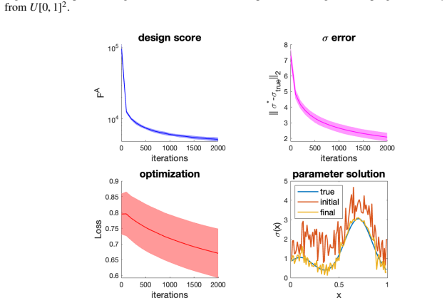
- In the Lorenz 63 tests, sampling at the algorithm-identified observation times converges faster and to lower reconstruction error than uniform sampling.
- In the Schrödinger tests, the optimized design concentrates source-detector pairs along the diagonal $\theta_1=\theta_2$, indicating that collocated measurements are most informative.
- Algorithm 2 lowers the per-iteration cost from $O(dNT')$ to $O(d^3+d^2N)$, making larger particle counts feasible.
Reading between the lines
- A natural next test is to compare this bilevel descent against the full gradient that includes the change of $\sigma^*$ with $\rho$; if the omitted term matters, the method may still succeed as an alternating heuristic rather than a true gradient method.
- The diagonal concentration found in the Schrödinger example suggests a transferable sensor-placement principle: when sources and detectors are local, coincident pairs dominate information, which could be probed in other inverse problems.
- The open convergence questions in the paper could be attacked empirically by fixing the time step, increasing $N$ and $T$, and checking whether the design measure approaches the benchmark ground-truth design computed with $\sigma = \sigma_{\mathrm{true}}$.
- The flat D-optimal density along the diagonal despite a varying potential hints that D-optimality is insensitive to the magnitude of the parameter field; verifying this on synthetic potentials with different contrast would clarify when A- and D-optimal designs differ.
Editorial analysis
A structured set of objections, weighed in public.
Referee Report
Summary. The paper develops a computational method for nonlinear optimal experimental design (OED) over a continuously indexed design space. It formulates the problem as a bilevel optimization (3) in which the outer level minimizes a design criterion F over a probability measure ρ on the design space, and the inner level computes the maximum-likelihood-type parameter estimate σ*[ρ] from the weighted loss (1). The proposed solvers, Algorithm 1 (brute-force inner loop) and Algorithm 2 (one-step streamlined inner update), move particles by a Wasserstein gradient-flow velocity and update σ* either by full inner optimization or by an implicit-function-theorem step. Numerical experiments on the Lorenz 63 system and a steady-state Schrödinger model show that the adaptive designs concentrate measurements at physically plausible times or locations and improve parameter reconstruction relative to uniform sampling. The paper claims in Section 1.2 to be the first to address nonlinear OED by optimizing a continuous design distribution in Pr2(Ω).
Significance. If the method is correct, it is a useful contribution to OED: it addresses a genuinely nonlinear, continuously indexed setting that most existing discrete-design or linear-model methods do not cover, and the particle/gradient-flow formulation is a natural way to avoid finite-dimensional design grids. The experimental comparisons on Lorenz 63 and the Schrödinger equation are valuable demonstrations of the type of design patterns the method can discover, and the paper is honest about the lack of convergence theory in Section 6. However, the paper's central mathematical claim—that Algorithms 1 and 2 are Wasserstein gradient flows for the stated bilevel objective—is not supported by the printed formulas, because the outer velocity omits the implicit derivative of σ* with respect to ρ. The numerical results may still support the method as a heuristic, but the gradient-flow interpretation and the associated optimality claims need repair.
major comments (4)
- [Section 3.2, Eqs. (15)-(16)] The paper labels (15) as the gradient flow of the reduced objective F[ρ;σ*[ρ]], but the velocity fields (16a)-(16b) are computed by differentiating F at a frozen σ and then evaluating at σ=σ*[ρ]. They omit the chain-rule term (∂F/∂σ)·Dρσ*[ρ] that arises from the implicit dependence of σ* on ρ. Therefore Algorithms 1 and 2 are not a Wasserstein gradient flow for the bilevel problem (3); they are an alternating design/parameter update heuristic. This is load-bearing for the central claim in Section 1.2. Please either compute the missing term and correct the velocities, or reframe the method as a heuristic and adjust the statements accordingly.
- [Section 3.2, Eqs. (17)-(18)] The signs in the particle update are inconsistent. Eq. (17) states θ̇_i = -∇_θ δF/δρ, while the forward-Euler update in (18) is θ_i^{t+1} = θ_i^t + Δt ∇_θ δF/δρ, with the minus sign omitted. This is not a harmless typo: the direction of particle motion and hence the entire algorithm depend on the sign. Please state the correct update and ensure that the implementation and the displayed formulas use the same sign.
- [Section 5, Eqs. (23)-(24)] The streamlined update in the Schrödinger experiments drops the second lines of both (23) and (24), i.e. the Hess_σ M and ∇_θ∇_σ M terms, with the rationale that the discrepancy M(θ;σ*)-data(θ) is small. No error estimate or numerical ablation is provided for this approximation. Since these terms carry second-order information about the nonlinear PtO map, the Schrödinger experiments demonstrate a simplified variant of Algorithm 2, not the full formula as written. Please provide a bound or a comparison showing that the dropped terms are negligible in the tested regime.
- [Section 6, limitation 1] The authors explicitly concede that convergence properties of Algorithm 2 are open. This alone would be acceptable for a numerical methods paper, but in combination with the omission of the chain-rule term in Major Comment 1, the lack of a descent guarantee is more serious: the empirical figures show that plotted objectives improve on the tested problems, yet there is no evidence that the iterates descend the reduced objective G(ρ)=F[ρ;σ*[ρ]]. The paper should either provide a monotonicity/descent statement for a corrected update or clearly characterize Algorithm 2 as a heuristic without a gradient interpretation.
minor comments (4)
- [Section 2.2, Eq. (8)] The set Γ(µ,ν) is used but not defined; please identify it as the set of couplings of µ and ν with the given marginals.
- [Section 4.2, warm-start A-optimal] The text sets '∆t = 50 1', which appears to be a typographical artifact; please clarify the intended step size.
- [Section 5.2, last paragraph] The sentence 'the top-right panel shows that the design score starts from a value much close to optimality' appears to refer to the wrong panel of Fig. 24; the top-right panel shows reconstruction error, not the design score. Please correct the cross-reference.
- [Section 6, limitation 2] The hyperparameters T, Δt, Δt', and T' are reported separately for each experiment but not collected in one place; a summary table would make the experiments easier to reproduce.
Circularity Check
No circularity: the design optimization and benchmarks are self-contained; the self-citation to [37] is not load-bearing.
full rationale
The paper's central derivation is not equivalent to its inputs by construction. Problem (3) is a genuine bilevel optimization over the design measure and the inferred parameter, and the algorithms alternate between a Wasserstein-gradient update of the particle design and an inner update of the parameter. The velocity formulas in (16a)-(16b) are stated as the nonlinear extension of the linear-case calculation in [37], but they follow by direct differentiation of the Fisher-information criteria (13), and no fitted constant or measured quantity is renamed as a prediction. The numerical validation is also non-circular: the benchmark designs in Figs. 3 and 10 are computed with fixed ground-truth parameters, independently of the adaptive outputs, and comparing the algorithm's design to that benchmark is a standard synthetic test rather than a self-referential evaluation. The only self-citation, [37], supplies an algebraic gradient-flow formula for the linear case; the present nonlinear extension is derived in the text and the central claim of solving continuous nonlinear OED does not rest on an unverified assertion from that citation. Section 6 explicitly concedes that no convergence theory is provided, so the empirical support is what carries the paper; that is a completeness or correctness limitation, not a circularity. The omission of the implicit derivative of sigma*[rho] in the outer velocity (Section 3.2) is a mathematical-flaw concern about whether Algorithm 2 is a true gradient flow for the reduced objective, but it is not an identity between inputs and outputs and therefore does not constitute circularity.
Assumptions & free parameters
free parameters (4)
- Outer step size Δt =
10^-5 to 5×10^1 across experiments
- Inner step size Δt' and inner iterations T' =
Δt' = 10^-5 to 10^-3; T' = 20 in Algorithm 1, 50 steps for initial σ*
- Particle count N and outer iterations T =
N from 18 to 10,000; T from 50 to 2,000
- Density threshold for identifying important time slots =
5%
assumptions (5)
- domain assumption The parameter-to-output map M(θ; σ) is sufficiently smooth for all derivatives used in the derivation.
- domain assumption The inner problem (1) has a unique global minimizer σ*[ρ] for every ρ, and the Hessian of the loss is invertible along the algorithm trajectory.
- domain assumption The Fisher information matrix I[ρ; σ] evaluated at the current reconstruction controls reconstruction error in the nonlinear setting as it does in the linear model.
- domain assumption Observed data are generated as data(θ) = M(θ; σ_true) + ε with Gaussian noise.
- ad hoc to paper In the Schrödinger experiments, σ* is close enough to σ_true that the second terms in (23) and (24) can be dropped.
Cite this review
Pith. "Pith review of Continuous nonlinear adaptive experimental design with gradient flow." pith.science (2026). https://pith.science/paper/LIY7US45
@misc{pith2026241114332,
  author       = {Pith},
  title        = {Pith review of: Continuous nonlinear adaptive experimental design with gradient flow},
  year         = {2026},
  howpublished = {\url{https://pith.science/paper/LIY7US45}},
  note         = {Machine review of arXiv:2411.14332}
}
read the original abstract
In computational inverse problems, the optimal experimental design (OED) problem seeks the best locations in time and space at which to take measurements. We investigate the nonlinear OED problem in the context of continuously-indexed design space for the measurements. In contrast to traditional approaches that select experiments from a finite measurement set, a continuous design space is often a better reflection of practical experimental options, where there is considerable flexibility concerning where and when to take measurements. The continuously-indexed space introduces computational challenges, and we address them by employing gradient-flow and optimal transport techniques, complemented by an adaptive strategy for bi-level optimization. Numerical results on the Lorenz 63 system and Schrodinger equation demonstrate that our solver identifies good measurement times / locations and achieves improved reconstruction of unknown parameters in inverse problems.
Figures


Figures from the paper (22 more)






Reference graph
Works this paper leans on
-
[1]
Alen Alexanderian. Optimal experimental design for infi nite-dimensional bayesian inverse problems governed by pdes: A review. Inverse Problems , 37(4):043001, 2021. 29
work page 2021
-
[2]
Alen Alexanderian, Noemi Petra, Georg Stadler, and Omar Ghattas. A-optimal design of experiments for infinite-dimensional bayesian li near inverse prob- lems with regularized ℓ0-sparsification. SIAM Journal on Scientific Computing , 36(5):A2122–A2148, 2014
work page 2014
-
[3]
Alen Alexanderian, Noemi Petra, Georg Stadler, and Omar Ghattas. A fast and scalable method for a-optimal design of experiments for infinite-dimensional bayesian nonlinear inverse problems. SIAM Journal on Scientific Computing , 38(1):A243–A272, 2016
work page 2016
-
[4]
E fficient d-optimal design of exper- iments for infinite-dimensional bayesian linear inverse pr oblems
Alen Alexanderian and Arvind K Saibaba. E fficient d-optimal design of exper- iments for infinite-dimensional bayesian linear inverse pr oblems. SIAM Journal on Scientific Computing , 40(5):A2956–A2985, 2018
work page 2018
-
[5]
Gradient flows: in metric spaces and in the space of probability measures
Luigi Ambrosio, Nicola Gigli, and Giuseppe Savar´ e. Gradient flows: in metric spaces and in the space of probability measures . Springer Science & Business Media, 2005
work page 2005
-
[6]
Introduction to optimum design
Jasbir Singh Arora. Introduction to optimum design . Elsevier, 2004
work page 2004
-
[7]
Gone fish- ing: Neural active learning with fisher embeddings
Jordan Ash, Surbhi Goel, Akshay Krishnamurthy, and Sham Kakade. Gone fish- ing: Neural active learning with fisher embeddings. In Advances in Neural In- formation Processing Systems, volume 34, pages 8927–8939. Curran Associates, Inc., 2021
work page 2021
-
[8]
Go al-oriented optimal design of experiments for large-scale bayesian linear inve rse problems
Ahmed Attia, Alen Alexanderian, and Arvind K Saibaba. Go al-oriented optimal design of experiments for large-scale bayesian linear inve rse problems. Inverse Problems, 34(9):095009, 2018
work page 2018
Show all 56 references
-
[9]
Optimal and e fficient designs of experiments
Corwin L Atwood. Optimal and e fficient designs of experiments. The Annals of Mathematical Statistics, pages 1570–1602, 1969
1969
-
[10]
Active perception
Ruzena Bajcsy. Active perception. Proceedings of the IEEE , 76(8):966–1005, 1988
1988
-
[11]
Schl¨ oder
Irene Bauer, Hans Georg Bock, Stefan K¨ orkel, and Johan nes P . Schl¨ oder. Nu- merical methods for optimum experimental design in dae syst ems. Journal of Computational and Applied Mathematics , 120(1):1–25, 2000
2000
-
[12]
Practic al considerations for optimal designs in clinical dose finding studies
Frank Bretz, Holger Dette, and Jose C Pinheiro. Practic al considerations for optimal designs in clinical dose finding studies. Statistics in medicine , 29(7- 8):731–742, 2010
2010
-
[13]
Minimax bounds for activ e learning
Rui M Castro and Robert D Nowak. Minimax bounds for activ e learning. IEEE Transactions on Information Theory, 54(5):2339–2353, 2008
2008
-
[14]
Bayesian Ex perimental Design: A Review
Kathryn Chaloner and Isabella V erdinelli. Bayesian Ex perimental Design: A Review. Statistical Science, 10(3):273 – 304, 1995. 30
1995
-
[15]
Convergence rates of active learning for maximum likelihoo d estimation
Kamalika Chaudhuri, Sham M Kakade, Praneeth Netrapall i, and Sujay Sanghavi. Convergence rates of active learning for maximum likelihoo d estimation. Ad- vances in Neural Information Processing Systems , 28, 2015
2015
-
[16]
Determina tion of a small elliptical anomaly in electrical impedance tomography using minimal measurements
Gaoming Chen, Fadil Santosa, and Aseel Titi. Determina tion of a small elliptical anomaly in electrical impedance tomography using minimal measurements. arXiv preprint arXiv:2403.11365, 2024
2024 arXiv
-
[17]
M.A. Clyde. Experimental design: Bayesian designs. In International Encyclo- pedia of the Social & Behavioral Sciences, pages 5075–5081. Pergamon, Oxford, 2001
2001
-
[18]
Optimal Design for Nonlinear Response Models
V alerii Fedorov and Sergei Leonov. Optimal Design for Nonlinear Response Models. 07 2013
2013
-
[19]
Model-oriented design of experiments , vol- ume 125
V alerii V Fedorov and Peter Hackl. Model-oriented design of experiments , vol- ume 125. Springer Science & Business Media, 2012
2012
-
[20]
Elsevier, 2013
V alerii V adimovich Fedorov.Theory of optimal experiments . Elsevier, 2013
2013
-
[21]
Figalli and F
A. Figalli and F. Glaudo. An Invitation to Optimal Transport, W asserstein Dis- tances, and Gradient Flows . EMS textbooks in mathematics. European Mathe- matical Society, 2021
2021
-
[22]
A unified stochastic gradient approach to design ing bayesian-optimal experiments
Adam Foster, Martin Jankowiak, Matthew O’Meara, Y ee Wh ye Teh, and Tom Rainforth. A unified stochastic gradient approach to design ing bayesian-optimal experiments. In International Conference on Artificial Intelligence and St atistics, pages 2959–2969. PMLR, 2020
2020
-
[23]
Deep Bayesian active learning with image data
Y arin Gal, Riashat Islam, and Zoubin Ghahramani. Deep Bayesian active learning with image data. In Doina Precup and Y ee Whye Teh, editors, Proceedings of the 34th International Conference on Machine Learning , volume 70 of Proceedings of Machine Learning Research, pages 1183...
2017
-
[24]
Nea r-optimal bayesian ac- tive learning with noisy observations
Daniel Golovin, Andreas Krause, and Debajyoti Ray. Nea r-optimal bayesian ac- tive learning with noisy observations. Advances in Neural Information Processing Systems, 23, 2010
2010
-
[25]
Introduction to quantum mechanics
David J Gri ffiths and Darrell F Schroeter. Introduction to quantum mechanics . Cambridge university press, 2018
2018
-
[26]
Numerical methods for e xperimental design of large-scale linear ill-posed inverse problems
E Haber, L Horesh, and L Tenorio. Numerical methods for e xperimental design of large-scale linear ill-posed inverse problems. Inverse Problems, 24(5):055012, sep 2008
2008
-
[27]
Numerical methods for t he design of large-scale nonlinear discrete ill-posed inverse problem s
E Haber, L Horesh, and L Tenorio. Numerical methods for t he design of large-scale nonlinear discrete ill-posed inverse problem s. Inverse Problems , 26(2):025002, 2009. 31
2009
-
[28]
Numeri- cal methods for a-optimal designs with a sparsity constrain t for ill-posed inverse problems
Eldad Haber, Zhuojun Magnant, Christian Lucero, and Lu is Tenorio. Numeri- cal methods for a-optimal designs with a sparsity constrain t for ill-posed inverse problems. Computational Optimization and Applications , 52:293–314, 2012
2012
-
[29]
Bayesian opti- mal designs for phase i clinical trials
Linda M Haines, Inna Perevozskaya, and William F Rosenb erger. Bayesian opti- mal designs for phase i clinical trials. Biometrics, 59(3):591–600, 2003
2003
-
[30]
Optimization with PDE Constraints, volume 23
Michael Hinze, Ren´ e Pinnau, Michael Ulbrich, and Stefan Ulbrich. Optimization with PDE Constraints, volume 23. Springer Science & Business Media, 2008
2008
-
[31]
Bayesian active learning for classification and preference learning
Neil Houlsby, Ferenc Husz´ ar, Zoubin Ghahramani, and M ´ at´ e Lengyel. Bayesian active learning for classification and preference learning . arXiv preprint arXiv:1112.5745, 2011
2011 arXiv
-
[32]
Optima l experimental design: Formulations and computations
Xun Huan, Jayanth Jagalur, and Y oussef Marzouk. Optima l experimental design: Formulations and computations. Acta Numerica, 33:715–840, 2024
2024
-
[33]
Simulation-based optim al bayesian ex- perimental design for nonlinear systems
Xun Huan and Y oussef M Marzouk. Simulation-based optim al bayesian ex- perimental design for nonlinear systems. Journal of Computational Physics , 232(1):288–317, 2013
2013
-
[34]
Gradient-based stochas tic optimization methods in bayesian experimental design
Xun Huan and Y oussef M Marzouk. Gradient-based stochas tic optimization methods in bayesian experimental design. International Journal for Uncertainty Quantification , 4(6), 2014
2014
-
[35]
Sequential bayesian opt imal ex- perimental design via approximate dynamic programming
Xun Huan and Y oussef M Marzouk. Sequential bayesian opt imal ex- perimental design via approximate dynamic programming. arXiv preprint arXiv:1604.08320, 2016
2016 arXiv
-
[36]
Batch gree dy maximization of non-submodular functions: Guarantees and applications to experimental design
Jayanth Jagalur-Mohan and Y oussef Marzouk. Batch gree dy maximization of non-submodular functions: Guarantees and applications to experimental design. The Journal of Machine Learning Research , 22(1):11397–11458, 2021
2021
-
[37]
Op timal experimental design for linear models via gradient flow
Ruhui Jin, Martin Guerra, Qin Li, and Stephen Wright. Op timal experimental design for linear models via gradient flow. arXiv preprint arXiv:2401.07806 , 2024
2024
-
[38]
Optimal designs for mi xed continuous and binary responses with quantitative and qualitative factors
Ming-Hung Kao and Hazar Khogeer. Optimal designs for mi xed continuous and binary responses with quantitative and qualitative factors. Journal of Multivariate Analysis, 182:104712, 2021
2021
-
[39]
J. Kiefer. General Equivalence Theory for Optimum Desi gns (Approximate The- ory). The Annals of Statistics , 2(5):849 – 879, 1974
1974
-
[40]
Kiefer and J
J. Kiefer and J. Wolfowitz. Optimum Designs in Regressi on Problems. The Annals of Mathematical Statistics , 30(2):271 – 294, 1959
1959
-
[41]
An introduction to the mathematical th eory of inverse problems
Andreas Kirsch. An introduction to the mathematical th eory of inverse problems. Applied Mathematical Sciences , 1996. 32
1996
-
[42]
The implicit function theorem: history, theory, and applications
Steven George Krantz and Harold R Parks. The implicit function theorem: history, theory, and applications. Springer Science & Business Media, 2002
2002
-
[43]
Nonlin ear bayesian opti- mal experimental design using logarithmic sobolev inequal ities
Fengyi Li, A youb Belhadji, and Y oussef Marzouk. Nonlin ear bayesian opti- mal experimental design using logarithmic sobolev inequal ities. arXiv preprint arXiv:2402.15053, 2024
2024 arXiv
-
[44]
Edward N. Lorenz. Deterministic nonperiodic flow. Journal of Atmospheric Sci- ences, 20(2):130 – 141, 1963
1963
-
[45]
Continuous-v ariable optical quantum-state tomography
Alexander I Lvovsky and Michael G Raymer. Continuous-v ariable optical quantum-state tomography. Reviews of modern physics , 81(1):299–332, 2009
2009
-
[46]
D-optimal
Toby J. Mitchell. An algorithm for the construction of “ D-optimal” experimental designs. T echnometrics, 42(1):48–54, 2000
2000
-
[47]
Active learning with expected error reduction
Stephen Mussmann, Julia Reisler, Daniel Tsai, Ehsan Mo usavi, Shayne O’Brien, and Moises Goldszmidt. Active learning with expected error reduction. arXiv preprint arXiv:2211.09283, 2022
2022 arXiv
-
[48]
Optimal Design of Experiments
Friedrich Pukelsheim. Optimal Design of Experiments. Society for Industrial and Applied Mathematics, 2006
2006
-
[49]
Design and analysis of computer experiments
Jerome Sacks, William J Welch, Toby J Mitchell, and Henr y P Wynn. Design and analysis of computer experiments. Statistical Science, 4(4):409–423, 1989
1989
-
[50]
Optimal Transport for Applied Mathematicians: Calculus of V ariations, PDEs, and Modeling, volume 87
Filippo Santambrogio. Optimal Transport for Applied Mathematicians: Calculus of V ariations, PDEs, and Modeling, volume 87. Birkh¨ auser, 2015
2015
-
[51]
Bayesian sequential optimal experimental design for linear regression with reinforcement learning
Fadil Santosa and Loren Anderson. Bayesian sequential optimal experimental design for linear regression with reinforcement learning. In 2022 21st IEEE In- ternational Conference on Machine Learning and Applicatio ns (ICMLA), pages 641–646, 2022
2022
-
[52]
Active learning for con volutional neural net- works: A core-set approach
Ozan Sener and Silvio Savarese. Active learning for con volutional neural net- works: A core-set approach. arXiv preprint arXiv:1708.00489 , 2017
2017 arXiv
-
[53]
Active learning literature survey
Burr Settles. Active learning literature survey. 2009
2009
-
[54]
Inverse problem theory and methods for model parameter esti - mation
Albert Tarantola. Inverse problem theory and methods for model parameter esti - mation. SIAM, 2005
2005
-
[55]
The sequential generation of d-optimum experimental designs
Henry P Wynn. The sequential generation of d-optimum experimental designs. The Annals of Mathematical Statistics , 41(5):1655–1664, 1970
1970
-
[56]
Mastering quantum mechanics: essentials, theory, and appl i- cations
Barton Zwiebach. Mastering quantum mechanics: essentials, theory, and appl i- cations. MIT Press, 2022. 33
2022
Reviewed August 12, 2026 · model on record in the stance chip above.
Discussion (0). Continue with ORCID to comment.