REVIEW 3 major objections 4 minor 49 references
Gradient-based optimization for variational empirical Bayes multiple regression
T0 review · 3 major / 4 minor · reviewed 2026-08-12 · deepseek-v4-flash
Pith's one-line read Replacing coordinate ascent with quasi-Newton steps keeps predictive accuracy, cuts iterations on correlated predictors, and reduces each optimization step to matrix-vector products.
desk verdict A practical, honest methods paper on gradient-based VEB regression; the compound-penalty trick is real, but the convergence claims are overreaching. read the letter →
The pith
A machine-rendered reading of the paper's core claim, the machinery that carries it, and where it could break.
The reading
What carries the argument
The central object is the normal-means posterior-mean operator $S_{g,v}(z)$, which maps a noisy observation $z$ to the posterior mean of the signal under prior $g$ and variance $v^2$; its inverse is denoted $T$. The penalized-regression theorem converts VEB into minimizing $\frac{1}{2\sigma^2}\|y - X\theta\|^2$ plus a sum of penalties $\rho(\theta_j, g, v_j^2)$, where the penalty satisfies $\rho'(\theta_j) = (T(\theta_j) - \theta_j)/v_j^2$. This identity means that the intractable penalty and its gradients can be evaluated from $T$ and the normal-means log marginal likelihood $\ell_{NM}$. The paper's two algorithms are two ways to compute $T$: Direct uses trisection-style numerical inversion, with a faster switch-and-spline inversion when $v_j$ is constant, and Compound reparameterizes through $z = T(\theta)$ to obtain an analytic penalty. A limited-memory quasi-Newton optimizer then minimizes either objective, so the dominant per-step work is the matrix-vector products $Xr$ and $X^T r$.
What would settle it
Take a spike-and-slab prior and compute $S_{g,v}(z)$ on a fine grid of $z$ values for several variances $v$; if any observed $\theta$ has more than one preimage under $S$, then the inverse $T$ used by both variants is not single-valued, and Direct's numerical inversion or Compound's reparameterization would fail on a regression with that prior.
Extended reading notes
Core claim
The paper builds on the result that variational empirical Bayes regression with a factorized posterior is exactly a penalized regression in the posterior mean $\theta$: minimizing $h(\theta, g, \sigma^2) = \frac{1}{2\sigma^2}\|y - X\theta\|^2 + \sum_j \rho(\theta_j, g, v_j^2) + \text{constants}$, where the penalty $\rho$ is defined through the normal-means posterior mean $S_{g,v}(z)$ and its inverse $T = S^{-1}$. The discovery is that this penalized regression objective can be optimized by quasi-Newton methods rather than coordinate updates, provided one can evaluate $T$. The Direct variant evaluates $T$ by numerical inversion at each evaluation; the Compound variant changes variables to $z = T(\theta)$ so that $\theta = S(z)$, making the compound penalty analytically tractable and avoiding inversion during optimization. The paper shows numerically that both variants match coordinate-ascent predictive accuracy, that the Compound variant often reaches a better ELBO in fewer iterations on block-correlated designs, and that in trend filtering the gradient methods complete far more iterations within the same time because the matrix-vector products $Xr$ and $X^T r$ exploit the structure of the design matrix.
Load-bearing premise
Everything rests on the assumption that the normal-means posterior-mean map $S$ can be inverted reliably on every value the optimizer visits: Direct numerically solves $S(z) = \theta$, and Compound assumes $\theta \mapsto S^{-1}(\theta)$ is a well-defined bijection, an assumption that is justified only for constant variances and otherwise relies on bracketing and monotonicity that the paper does not verify.
Editorial extensions
If this is right
- Any design matrix with a fast multiplication routine, such as trend filtering, Fourier or wavelet bases, or sparse graphs, becomes a setting where GradVI is much faster than coordinate ascent, because both objective and gradient evaluations reduce to $Xr$ and $X^T r$ products.
- For correlated predictors, GradVI with a null initialization can match or beat coordinate ascent initialized from a lasso fit, which removes the costly cross-validation step that large regression problems currently require.
- The modular treatment of priors means that adding a new prior family only requires solving the corresponding normal-means problem, rather than deriving and debugging full coordinate updates for that prior.
- In Bayesian trend filtering, the paper reports better estimates of changepoint magnitudes than cross-validated $\ell_1$ trend filtering, especially at high noise, and reports scalability to $n = 10^6$ observations on a single machine.
- The gradient-based structure can exploit parallel and GPU-accelerated matrix multiplication in ways that sequential coordinate ascent cannot.
Reading between the lines
- The same penalized-regression reformulation should extend beyond normal means: any variational family whose mean map has a tractable inverse would let GradVI-style optimization handle non-Gaussian likelihoods, such as logistic regression, a natural extension the paper does not test.
- Because the cost is dominated by matrix-vector products, GradVI could be combined with randomized linear algebra, sketching, or fast transforms to attack designs that are too large to store explicitly.
- The Compound variant's reliance on a bijective map $S$ suggests a practical diagnostic: before using it with a new prior, one should check monotonicity of $S$ over the range of $v_j$ values that arise in optimization, since the paper only gives a monotonicity argument for constant $v_j$.
- The comparison with cross-validated $\ell_1$ trend filtering hints at a general phenomenon: empirical-Bayes penalties that estimate component sizes from data may recover signal magnitudes that a single $\ell_1$ penalty systematically shrinks.
Editorial analysis
A structured set of objections, weighed in public.
Referee Report
Summary. The paper proposes GradVI, a quasi-Newton (L-BFGS-B) alternative to coordinate-ascent variational inference (CAVI) for fitting variational empirical Bayes sparse multiple regression with normal-mixture priors. It builds on the Kim et al. penalized-likelihood reformulation of the VEB objective, and develops two implementations: Direct (numerically inverting the posterior mean operator) and Compound (reparameterizing via the inverse operator). The paper reports simulation comparisons in high-dimensional regression and zeroth-order trend filtering, and claims that GradVI matches CAVI accuracy, converges in fewer iterations under correlated predictors, and is much faster when fast matrix-vector products are available. The central mathematical identities are the derivative formulas (22)-(24) and the compound objective (25).
Significance. If the claims held, GradVI would be a useful and flexible algorithmic contribution: it reduces the per-iteration cost to matrix-vector products, accommodates automatic differentiation and new priors, and the authors provide open-source code and reproducible DSC pipelines. The derivative identities follow from Tweedie's formula, and the PLR theorem is a published result from Kim et al., so the derivation is not circular. The practical significance is currently only partially established, however, because several empirical comparisons lack a converged baseline and the recommended variant sometimes fails to converge within the iteration budget.
major comments (3)
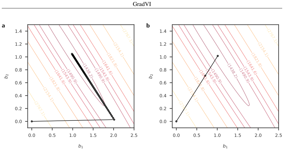
- [Sec. 4.2, Fig. 2 (right column); Fig. 5] The trend-filtering experiments do not establish the abstract's claim that GradVI 'converges in fewer iterations' or 'is much faster than CAVI' in settings with fast matrix-vector products. The text states that CAVI did not converge within 2000 iterations on the unscaled H matrix, that GradVI Compound did not converge within 2000 iterations on the scaled H matrix, and that the ELBO/RMSE 'reference' is a non-converged CAVI run. The scaled-H comparison also changes the design matrix and hence the induced prior on the regression coefficients, so ELBO values across scaled and unscaled runs are not directly comparable. Please report convergence rates for every method/design, compare against a converged baseline (for example, a longer CAVI run or a smaller ELBO tolerance), or explicitly qualify the speed and iteration claims as applying only to runs that terminate.
- [Sec. 4.1 (Block-correlated variables); Sec. 5] The recommendation of Compound as the default is undercut by its failure to converge in some correlated-predictor simulations. The text reports 'GradVI Compound sometimes failed to converge after 2000 iterations, whereas GradVI Direct converged in all simulations.' Because the abstract's 'converges in fewer iterations when the predictors are highly correlated' claim is based on these simulations, the paper must report how often each variant fails, the distribution of iteration counts conditional on convergence, and whether the iteration summaries in Fig. 2 include non-converged runs (for example, censored at 2000). Without this, the claim holds only for a selected subset of runs.
- [Sec. 3.1 and 3.2, Eqs. (19)-(25)] The existence and properties of the inverse operator T = S^{-1} are assumed rather than proved for the general case. Symmetry and monotonicity are asserted only for constant v_j, yet the Direct method applies trisection for coordinate-dependent v_j and the Compound reparameterization z = T(theta) requires T to be a bijection over the relevant range. Please provide a proof (or precise conditions) that S_{g,v_j} is strictly increasing and onto for the ash and point-normal priors used here, and give bracketing/error guarantees for the trisection inversion. If such a guarantee is not available, state the resulting limitation explicitly.
minor comments (4)
- [Sec. 3.1 and Sec. 3.2] There are several typos, including 'optimzation' in Sec. 3.1 and 'tractible' in Secs. 3.2 and 5; please correct them.
- [Sec. 2.1] The notation paragraph says vectors are denoted by bold lowercase letters with 'e.g., b', but then writes 'e.g., y or Y'; please make the vector/scalar notation for y consistent.
- [Sec. 4.2 and Fig. 4] The text refers to panels (a), (b), and (c) of Fig. 4, but the figure as described does not show clear panel labels; please add labels to the figure panels.
- [Sec. 5] The Discussion claims GradVI 'enables trend filtering for datasets with n = 10^6 on a single core with 100 GB of memory,' but no experiment in the manuscript supports this; please indicate whether this is a reported run or an extrapolation.
Circularity Check
No significant circularity: the central derivation rests on an independently published PLR theorem, and the validation is an optimizer comparison on a shared objective, not a fitted quantity renamed as a prediction.
full rationale
The paper's load-bearing derivation is the PLR theorem of Kim et al. [29], which rewrites the variational empirical Bayes objective (8) as a penalized regression objective (14)-(15). This theorem is a published mathematical result with its own derivation; although it comes from the same research group, it does not assume the conclusions of this paper, and the paper does not fit parameters to data and then rename those fitted values as predictions. The two GradVI variants are optimization strategies for that shared objective, and the comparisons against CAVI are comparisons of optimizers on the same objective, which is not circular. The manuscript explicitly reports limitations that weaken some headline claims: GradVI Compound sometimes failed to converge after 2000 iterations (Sec. 4.1), CAVI did not converge on the unscaled trend-filtering design, and the GradVI method did not converge on the scaled design, with the 'reference' ELBO coming from a non-converged CAVI run (Sec. 4.2). These are correctness or over-claiming concerns, not circularity: the paper is candid about the nonconvergence rather than using it to define its own success. The numerical inversion and trisection steps are implementation choices with stated assumptions, and no equation in the paper reduces to its own input by construction. The self-citation to [29] is load-bearing but is independent support in the sense of the review rules, because the PLR theorem is a stated, externally checkable mathematical result. Overall, no circular step was identified and the central claim has independent content.
Assumptions & free parameters
free parameters (3)
- ash mixture proportions w_k =
estimated from data
- residual variance sigma^2 =
estimated from data
- ash grid parameters K and sigma^2_k =
K=20, sigma^2_k=(2^((k-1)/20)-1)^2
assumptions (5)
- standard math PLR theorem of Kim et al. [29] (Eq. 14-18): the VEB objective can be written as a penalized regression over the posterior mean theta with penalty rho defined via the normal-means posterior mean operator S.
- domain assumption Mean-field factorization Q = product_j q_j(b_j) (Eq. 9).
- ad hoc to paper The posterior mean operator S_{g,v}(z) is invertible (monotone and surjective) for the priors used, so T=S^{-1} exists and the compound reparametrization is valid.
- standard math Tweedie's formula (13) connecting S and l'_NM.
- domain assumption For any prior g in G, l_NM and S are analytically tractable ([29], Sec. 2.4).
Cite this review
Pith. "Pith review of Gradient-based optimization for variational empirical Bayes multiple regression." pith.science (2026). https://pith.science/paper/IOI3AIMS
@misc{pith2026241114570,
  author       = {Pith},
  title        = {Pith review of: Gradient-based optimization for variational empirical Bayes multiple regression},
  year         = {2026},
  howpublished = {\url{https://pith.science/paper/IOI3AIMS}},
  note         = {Machine review of arXiv:2411.14570}
}
read the original abstract
Variational empirical Bayes (VEB) methods provide a practically attractive approach to fitting large, sparse, multiple regression models. These methods usually use coordinate ascent to optimize the variational objective function, an approach known as coordinate ascent variational inference (CAVI). Here we propose alternative optimization approaches based on gradient-based (quasi-Newton) methods, which we call gradient-based variational inference (GradVI). GradVI exploits a recent result from Kim et. al. [arXiv:2208.10910] which writes the VEB regression objective function as a penalized regression. Unfortunately the penalty function is not available in closed form, and we present and compare two approaches to dealing with this problem. In simple situations where CAVI performs well, we show that GradVI produces similar predictive performance, and GradVI converges in fewer iterations when the predictors are highly correlated. Furthermore, unlike CAVI, the key computations in GradVI are simple matrix-vector products, and so GradVI is much faster than CAVI in settings where the design matrix admits fast matrix-vector products (e.g., as we show here, trendfiltering applications) and lends itself to parallelized implementations in ways that CAVI does not. GradVI is also very flexible, and could exploit automatic differentiation to easily implement different prior families. Our methods are implemented in an open-source Python software, GradVI (available from https://github.com/stephenslab/gradvi ).
Figures


Figures from the paper (2 more)


Reference graph
Works this paper leans on
-
[1]
S. M. Stigler. “Studies in the history of probability and statistics XL Boscovich, Simpson and a 1760 manuscript note on fitting a linear relation”. Biometrika 71.3 (1984), pp. 615–620. D O I: 10.1093/biomet/71.3.615
-
[2]
Statistical challenges of high-dimensional data
I. M. Johnstone and D. M. Titterington. “Statistical challenges of high-dimensional data”. Philosophical Transac- tions of the Royal Society A: Mathematical, Physical and Engineering Sciences 367.1906 (2009), pp. 4237–4253. D O I: 10.1098/rsta.2009.0159
arXiv 2009
-
[3]
Statistical learning with sparsity
T. Hastie, R. Tibshirani, and M. Wainwright. “Statistical learning with sparsity”.Monographs on statistics and applied probability 143.143 (2015), p. 8
work page 2015
-
[4]
S.-J. Kim et al. “ ℓ1 Trend Filtering”. SIAM Review 51.2 (2009), pp. 339–360
work page 2009
-
[5]
Adaptive piecewise polynomial estimation via trend filtering
R. J. Tibshirani. “Adaptive piecewise polynomial estimation via trend filtering”. The Annals of Statistics 42.1 (2014), pp. 285–323. D O I: 10.1214/13-AOS1189
-
[6]
E. D. Feigelson and G. J. Babu. Modern statistical methods for astronomy: with R applications . Cambridge University Press, 2012
work page 2012
-
[7]
H. V on Storch and F. W. Zwiers.Statistical analysis in climate research. Cambridge university press, 2002
work page 2002
-
[8]
High-Dimensional Statistics with a View Toward Applications in Biology
P. Bühlmann, M. Kalisch, and L. Meier. “High-Dimensional Statistics with a View Toward Applications in Biology”. Annual Review of Statistics and Its Application 1.V olume 1, 2014 (2014), pp. 255–278.D O I: https: //doi.org/10.1146/annurev-statistics-022513-115545
Show all 49 references
-
[9]
R. S. Tsay. Analysis of financial time series. John Eiley and Sons, 2005
2005
-
[10]
Economic Predictions With Big Data: The Illusion of Sparsity
D. Giannone, M. Lenza, and G. E. Primiceri. “Economic Predictions With Big Data: The Illusion of Sparsity”. Econometrica 89.5 (2021), pp. 2409–2437. D O I: https://doi.org/10.3982/ECTA17842
2021 doi
-
[11]
Bayesian Variable Selection Regression for Genome-wide Association Studies and Other Large-Scale Problems
Y . Guan and M. Stephens. “Bayesian Variable Selection Regression for Genome-wide Association Studies and Other Large-Scale Problems”. The Annals of Applied Statistics 5.3 (2011), pp. 1780–1815
2011
-
[12]
Scalable Variational Inference for Bayesian Variable Selection in Regression, and Its Accuracy in Genetic Association Studies
P. Carbonetto and M. Stephens. “Scalable Variational Inference for Bayesian Variable Selection in Regression, and Its Accuracy in Genetic Association Studies”. Bayesian Analysis 7.1 (2012), pp. 73–108. D O I: 10.1214/ 12-BA703
2012
-
[13]
A Simple New Approach to Variable Selection in Regression, with Application to Genetic Fine Mapping
G. Wang et al. “A Simple New Approach to Variable Selection in Regression, with Application to Genetic Fine Mapping”. Journal of the Royal Statistical Society Series B: Statistical Methodology 82.5 (2020), pp. 1273–1300. D O I: 10.1111/rssb.12388
2020 doi
-
[14]
Polygenic Modeling with Bayesian Sparse Linear Mixed Models
X. Zhou, P. Carbonetto, and M. Stephens. “Polygenic Modeling with Bayesian Sparse Linear Mixed Models”. PLOS Genetics 9.2 (2013), pp. 1–14. D O I: 10.1371/journal.pgen.1003264
2013 doi
-
[15]
A fast and scalable framework for large-scale and ultrahigh-dimensional sparse regression with appli- cation to the UK Biobank
J. Qian et al. “A fast and scalable framework for large-scale and ultrahigh-dimensional sparse regression with appli- cation to the UK Biobank”. PLOS Genetics 16.10 (2020), pp. 1–30. D O I: 10.1371/journal.pgen.1009141. 14 GradVI
2020 doi
-
[16]
D. Gubbins. Time series analysis and inverse theory for geophysicists. Cambridge university press, 2004
2004
-
[17]
Gene selection in cancer classification using sparse logistic regression with Bayesian regularization
G. C. Cawley and N. L. C. Talbot. “Gene selection in cancer classification using sparse logistic regression with Bayesian regularization”. Bioinformatics 22.19 (2006), pp. 2348–2355. D O I: 10.1093/bioinformatics/ btl386
2006 doi
-
[18]
On Time Series Analysis of Public Health and Biomedical Data
S. L. Zeger, R. Irizarry, and R. D. Peng. “On Time Series Analysis of Public Health and Biomedical Data”.Annual Review of Public Health 27.V olume 27, 2006 (2006), pp. 57–79.D O I: https://doi.org/10.1146/annurev. publhealth.26.021304.144517
2006
-
[19]
Building Better Models: Prediction, Replication, and Machine Learning in the Social Sciences
M. Hindman. “Building Better Models: Prediction, Replication, and Machine Learning in the Social Sciences”. The ANNALS of the American Academy of Political and Social Science 659.1 (2015), pp. 48–62. D O I: 10.1177/ 0002716215570279
2015
-
[20]
Text Regression Analysis: A Review, Empirical, and Experimental Insights
K. Taha. “Text Regression Analysis: A Review, Empirical, and Experimental Insights”.IEEE Access 12 (2024), pp. 137333–137344. D O I: 10.1109/ACCESS.2024.3446765
2024
-
[21]
Ridge Regression: Biased Estimation for Nonorthogonal Problems
A. E. Hoerl and R. W. Kennard. “Ridge Regression: Biased Estimation for Nonorthogonal Problems”. Technomet- rics 12.1 (1970), pp. 55–67. D O I: 10.1080/00401706.1970.10488634
1970
-
[22]
Regression Shrinkage and Selection via the Lasso
R. Tibshirani. “Regression Shrinkage and Selection via the Lasso”. Journal of the Royal Statistical Society. Series B (Methodological) 58.1 (1996), pp. 267–288
1996
-
[23]
Regularization and Variable Selection Via the Elastic Net
H. Zou and T. Hastie. “Regularization and Variable Selection Via the Elastic Net”.Journal of the Royal Statistical Society Series B: Statistical Methodology67.2 (2005), pp. 301–320. D O I: 10.1111/j.1467-9868.2005.00503. x
2005
-
[24]
Bayesian Variable Selection in Linear Regression
T. J. Mitchell and J. J. Beauchamp. “Bayesian Variable Selection in Linear Regression”.Journal of the American Statistical Association 83.404 (1988), pp. 1023–1032. D O I: 10.1080/01621459.1988.10478694
1988
-
[25]
Variable Selection via Gibbs Sampling
E. I. George and R. E. McCulloch. “Variable Selection via Gibbs Sampling”. Journal of the American Statistical Association 88.423 (1993), pp. 881–889. D O I: 10.1080/01621459.1993.10476353
1993
-
[26]
The Bayesian Lasso
T. Park and G. Casella. “The Bayesian Lasso”. Journal of the American Statistical Association 103.482 (2008), pp. 681–686. D O I: 10.1198/016214508000000337
2008 doi
-
[27]
The Bayesian elastic net
Q. Li and N. Lin. “The Bayesian elastic net”. Bayesian Analysis 5.1 (2010), pp. 151–170. D O I: 10.1214/ 10-BA506
2010
-
[28]
False discovery rates: a new deal
M. Stephens. “False discovery rates: a new deal”. Biostatistics 18.2 (2016), pp. 275–294. D O I: 10.1093/ biostatistics/kxw041
2016
-
[29]
A flexible empirical Bayes approach to multiple linear regression and connections with penalized regression
Y . Kim et al. “A flexible empirical Bayes approach to multiple linear regression and connections with penalized regression”. Journal of Machine Learning Research 25.185 (2024), pp. 1–59
2024
-
[30]
Regularization Paths for Generalized Linear Models via Coordinate Descent
J. H. Friedman, T. Hastie, and R. Tibshirani. “Regularization Paths for Generalized Linear Models via Coordinate Descent”. Journal of Statistical Software 33.1 (2010), pp. 1–22. D O I: 10.18637/jss.v033.i01
2010 doi
-
[31]
Ridge Estimators in Logistic Regression
S. le Cessie and J. C. van Houwelingen. “Ridge Estimators in Logistic Regression”.Journal of the Royal Statistical Society: Series C (Applied Statistics) 41.1 (1992), pp. 191–201. D O I: https://doi.org/10.2307/2347628
1992 doi
-
[32]
An algorithm for quadratic programming
M. Frank and P. Wolfe. “An algorithm for quadratic programming”.Naval Research Logistics Quarterly 3.1-2 (1956), pp. 95–110. D O I: https://doi.org/10.1002/nav.3800030109
1956 doi
-
[33]
Solving large scale linear prediction problems using stochastic gradient descent algorithms
T. Zhang. “Solving large scale linear prediction problems using stochastic gradient descent algorithms”. Pro- ceedings of the Twenty-First International Conference on Machine Learning. ICML ’04. Banff, Alberta, Canada: Association for Computing Machinery, 2004, p. 116. D O I: ...
2004
-
[34]
Nocedal and S
J. Nocedal and S. Wright. Numerical Optimization. Springer Series in Operations Research and Financial Engineering. Springer New York, 2006
2006
-
[35]
Variable Metric Method for Minimization
W. C. Davidon. “Variable Metric Method for Minimization” (1959). D O I: 10.2172/4252678
1959 doi
-
[36]
Variable Metric Method for Minimization
W. C. Davidon. “Variable Metric Method for Minimization”.SIAM Journal on Optimization 1.1 (1991), pp. 1–17. D O I: 10.1137/0801001
1991 doi
-
[37]
C. M. Bishop. Pattern Recognition and Machine Learning. Springer-Verlag, 2006
2006
-
[38]
On information and sufficiency
S. Kullback and R. A. Leibler. “On information and sufficiency”.Annals of Mathematical Statistics 22.1 (1951), pp. 79–86
1951
-
[39]
An Introduction to Variational Methods for Graphical Models
M. I. Jordan et al. “An Introduction to Variational Methods for Graphical Models”.Machine Learning 37.2 (1999), pp. 183–233. D O I: 10.1023/A:1007665907178. 15 GradVI
1999 doi
-
[40]
Variational Inference: A Review for Statisticians
D. M. Blei, A. Kucukelbir, and J. D. McAuliffe. “Variational Inference: A Review for Statisticians”.Journal of the American Statistical Association 112.518 (2017), pp. 859–877. D O I: 10.1080/01621459.2017.1285773
2017
-
[41]
Proceedings of the Third Berkeley Symposium on Mathematical Statistics and Probability, vol. 1: Contributions to the Theory of Statistics
H. Robbins. “Proceedings of the Third Berkeley Symposium on Mathematical Statistics and Probability, vol. 1: Contributions to the Theory of Statistics” (1956)
1956
-
[42]
Trisection algorithms
N. Shammas. “Trisection algorithms”. HP Handheld Conference. 2014
2014
-
[43]
Fast Switch and Spline Function Inversion Algorithm with Multistep Optimiza- tion and k-Vector Search for Solving Kepler’s Equation in Celestial Mechanics
D. Tommasini and D. N. Olivieri. “Fast Switch and Spline Function Inversion Algorithm with Multistep Optimiza- tion and k-Vector Search for Solving Kepler’s Equation in Celestial Mechanics”.Mathematics 8.11 (2020). D O I: 10.3390/math8112017
2020 doi
-
[44]
On the limited memory BFGS method for large scale optimization
D. C. Liu and J. Nocedal. “On the limited memory BFGS method for large scale optimization”. Mathematical Programming 45.1 (1989), pp. 503–528. D O I: 10.1007/BF01589116
1989 doi
-
[45]
A Limited Memory Algorithm for Bound Constrained Optimization
R. H. Byrd et al. “A Limited Memory Algorithm for Bound Constrained Optimization”.SIAM Journal on Scientific Computing 16.5 (1995), pp. 1190–1208
1995
-
[46]
Algorithm 778: L-BFGS-B: Fortran subroutines for large-scale bound-constrained optimization
C. Zhu et al. “Algorithm 778: L-BFGS-B: Fortran subroutines for large-scale bound-constrained optimization”. ACM Trans. Math. Softw.23.4 (1997), pp. 550–560. D O I: 10.1145/279232.279236
1997
-
[47]
Stochastic Variational Inference
M. D. Hoffman et al. “Stochastic Variational Inference”. Journal of Machine Learning Research 14.4 (2013), pp. 1303–1347
2013
-
[48]
Black Box Variational Inference
R. Ranganath, S. Gerrish, and D. Blei. “Black Box Variational Inference”. Proceedings of the Seventeenth International Conference on Artificial Intelligence and Statistics . Ed. by S. Kaski and J. Corander. V ol. 33. Proceedings of Machine Learning Research. Reykjavik, Iceland...
2014
-
[49]
Automatic Differentiation Variational Inference
A. Kucukelbir et al. “Automatic Differentiation Variational Inference”.Journal of Machine Learning Research 18.14 (2017), pp. 1–45. 16
2017
Reviewed August 12, 2026 · model on record in the stance chip above.
Discussion (0). Continue with ORCID to comment.