REVIEW 4 major objections 6 minor 5 references
Bayesian optimal change point detection in high-dimensions
T0 review · 4 major / 6 minor · reviewed 2026-08-12 · deepseek-v4-flash
Pith's one-line read The paper proposes the first Bayesian change point detection methods for high-dimensional mean and covariance structures, proving consistency under milder conditions and near-minimax localization rates.
desk verdict A genuine first Bayesian method for high-dimensional change point detection, but the implemented alpha-calibration step falls outside the theorem conditions, so the consistency claims are conditional. read the letter →
The pith
A machine-rendered reading of the paper's core claim, the machinery that carries it, and where it could break.
The reading
What carries the argument
The central object is the maximum pairwise Bayes factor (mxPBF): for each candidate location $l$ and window size $n_w$, compute a Bayes factor for a change in each coordinate (mean case) or each pair of coordinates conditional on one another (covariance case) using only the $n_w$ observations before and after $l$, then take the maximum over coordinates or pairs and over candidate locations. The priors are centered at local sample means or local regression coefficients with variance scaled by $\gamma_{n_w} = (n_w \vee p)^{-\alpha}$, which makes the log Bayes factors grow or shrink at polynomial rates in $n_w \vee p$. The theory combines tail bounds on these pairwise Bayes factors with union bounds over locations and coordinates; the multiscale variant groups detections from several window sizes by a majority vote, and the localization guarantee follows because the refined estimate is chosen as the argmax within the window after the first threshold crossing.
What would settle it
Simulate from the null hypothesis $X_i \sim N_p(0, I_p)$ with $n = 500$, $p = 1000$, window $n_w = 50$, threshold $C_{cp} = 10$, and $\alpha$ chosen by the paper's FPR calibration with $N = 300$; if the proportion of null datasets in which the mxPBF exceeds $C_{cp}$ grows with $p$ instead of staying near the calibrated 0.05, then the implemented version does not have the null consistency that Theorem 2.1 claims for the theoretical $\alpha$.
Extended reading notes
Core claim
The paper establishes that change points in the mean vector or covariance matrix of a high-dimensional Gaussian sequence can be detected and localized by a maximum pairwise Bayes factor computed on small windows around each candidate location. For the mean, Theorems 2.1 and 2.2 prove that the test is consistent and that the estimated number and locations satisfy $P_0(\hat K = K_0, \max_k |i_k - \hat i_k| \le n_w) \to 1$ whenever the minimum scaled componentwise signal exceeds roughly $\log(n_w \vee p)/n_w$ and certain window, sparsity, and hyperparameter conditions hold; Theorem 2.3 gives a matching minimax lower bound up to a logarithmic factor. For the covariance, Theorems 3.1 and 3.2 give analogous guarantees under signal conditions (A3) or (A3*), and Theorems 3.3 and 3.4 show that the localization rate $n_w/n$ is minimax-optimal up to $\log(n_w \vee p)$. The authors contend that this is the first Bayesian treatment of high-dimensional change point detection and that its conditions are weaker than those of existing frequentist approaches, in particular allowing a fixed number of changed components and requiring no sparsity of precision matrices.
Load-bearing premise
The theorems guarantee consistency only for hyperparameter $\alpha$ satisfying explicit inequalities, but the implemented method selects $\alpha$ by simulating datasets from the sample mean and covariance and picking the value whose empirical false positive rate is below 0.05; the paper does not prove that this data-driven $\alpha$ satisfies the theoretical conditions, so the practical procedure may run outside the regime where consistency and near-optimality are proven.
Editorial extensions
If this is right
- For mean changes, consistent localization within $n_w$ is guaranteed provided each change point is separated by at least $n_w$ and some coordinate moves by at least $C \log(n_w \vee p)/n_w$ in standardized units; the number of changed coordinates may be fixed, which existing sparse-alternative tests do not allow.
- The localization error $n_w/n$ is minimax up to a logarithmic factor for single mean changes and for covariance changes under the stated signal classes, so the chosen window size directly sets the time resolution one can promise.
- Covariance detection requires no sparsity of the precision matrix and no irrepresentability condition, unlike earlier tests that estimated sparse precisions.
- The multiscale majority-vote version stabilizes detection across window choices, provided at least half of the window sizes satisfy the theorem conditions and the window ladder grows geometrically.
- On real data, running the covariance detector first and then the mean detector within segments yields change points that align with known financial and genomic events in the two reported applications.
Reading between the lines
- The modularization into per-coordinate or per-pair Bayes factors suggests the same windowed maximum test could be applied to sub-Gaussian or heavy-tailed data after robustifying the variance estimators, but the paper's proofs rely on exact Gaussian likelihoods, so the calibration of the log Bayes factor outside normality is unverified.
- Because the theory only requires one coordinate or pair with signal above the threshold, the method is intrinsically a maximum-type detector; the paper's own discussion notes it may miss many small coordinated changes, so a hybrid that first aggregates weak signals and then applies mxPBF is a natural testable extension.
- The FPR-based $\alpha$ calibration simulates from the plug-in Gaussian fit; a reader who wants to deploy the method should treat the consistency theorems as conditional on $\alpha$ satisfying the stated inequalities and verify the calibration on their own null model.
- The multiscale majority rule is proven only for window ladders with $n_w^{(r)} \le n_w^{(r+1)}/2$ and at least half of the windows meeting the theorem conditions; in practice, the stability of detected change points across window ladders could serve as a data-driven check.
Editorial analysis
A structured set of objections, weighed in public.
Referee Report
Summary. The paper proposes new Bayesian tests and change-point estimators for high-dimensional Gaussian sequences, using maximum pairwise Bayes factors computed in local windows. For mean changes it establishes consistency of the mxPBF test (Theorem 2.1), consistent estimation of the number and locations with error nw (Theorem 2.2), and a minimax lower bound showing near-optimal localization (Theorem 2.3). Analogous results are given for covariance changes (Theorems 3.1-3.4) under conditions (A2)-(A3*). The paper also proposes a multiscale majority-voting implementation, reports simulations comparing with Dette, Geomcp, Inspect, and Edivisive, and applies the methods to CGH and S&P 500 data. The theoretical results are stated for fixed alpha satisfying condition (7) or alpha > 6C3, while the implementation selects alpha by empirical false-positive calibration.
Significance. If the theorems are correct, the contributions are significant: they appear to be the first Bayesian change-point methods for high-dimensional mean and covariance structures with consistency under weaker sparsity and segment-length conditions than several frequentist competitors, and with near-minimax localization rates. The paper also includes explicit minimax lower-bound constructions, a public GitHub implementation, and comparisons with four existing methods. The modularized pairwise-Bayes-factor construction is computationally attractive because it avoids p-by-p matrix inversions. However, the main theorems are not self-contained, and the implemented tuning procedure is not covered by the theoretical guarantees; these issues must be addressed before the headline claims can be accepted.
major comments (4)
- [Section 4.2 and Appendix B; Theorems 2.1-2.2 and 3.1-3.2] The implemented method is not the version covered by the main theorems. Theorems 2.1, 2.2, 3.1, and 3.2 require a fixed alpha satisfying condition (7) in the mean case or alpha > 6C3 in the covariance case, whereas Section 4.2 and Appendix B select alpha by empirical false-positive calibration: N=300 datasets are simulated from N_p(mu-hat, Sigma-hat), where mu-hat and Sigma-hat are the sample mean and covariance of the observed data, and alpha is chosen so that the simulated mxPBF exceeds C_th with frequency below 0.05. No result in the paper shows that this data-dependent alpha-hat satisfies condition (7) or alpha-hat > 6C3, nor that simulating from the plug-in N_p(mu-hat, Sigma-hat) is a valid null distribution when change points are present; in the covariance-change case the pooled Sigma-hat is not the null covariance. A parallel gap exists for the covariance prior constants a0, b0, b01, b02, which are fixed at 0.01 in Section 4.2 without checking the inequalities in conditions (A3) and (A3*). Consequently, the Abstract's consistency and near-optimal localization claims apply to a version of the algorithm that is not the one run in the simulations or applied to the real datasets.
- [Appendix D, proofs of Theorems 2.1 and 3.1] The key probability bounds are not proved or stated in the paper. The proofs repeatedly invoke 'the proof of Theorem 2.1 in Lee et al. (2024)' or 'the proof of Theorem 3.1 in Lee et al. (2024)' to obtain tail bounds of the form (nw or p)^{-C} for the pairwise Bayes factors. These tail bounds are exactly what powers the null and alternative consistency arguments, and they are the source of the constants C1, C2, C3, Cbm, Cbm,a and of condition (7). As written, the main theorems are not self-contained: a reader cannot verify that the quoted lemmas hold under the paper's priors, windowing setup, and high-dimensional scaling without consulting an external manuscript. The needed lemmas should be stated and proved, or at least precisely stated with assumptions sufficient for the present paper.
- [Proof of Theorem 3.2, Appendix D.2] The final bound in the proof of Theorem 3.2 says that a sum over K0 change points is at most 14 K0 (nw or p)^{-C} = o(1) for some constant 2 < C < C1. But Theorem 3.2 defines C1 as a constant arbitrarily close to, but slightly larger than, 1, so the interval (2, C1) is empty and the inequality is vacuous. The preceding step also needs an explicit relationship between C and C1,low to justify the o(1) conclusion from the assumption K0(nw or p)^{-C1,low} = o(1). This makes the proof of Theorem 3.2 invalid as written, although the theorem may be salvageable with corrected constant comparisons.
- [Section 4.1, multiscale method] The multiscale 'mxPBF major' procedure is the method used in all simulations and real-data applications, but its theoretical justification is only a heuristic sentence: if at least the window sizes n_w^(1), ..., n_w^((|N|+1)/2) satisfy the conditions of Theorems 2.2 and 3.2 and n_w^(r) <= n_w^(r+1)/2, then 'it can be shown' that the localization rate is at most n_w^((|N|+1)/2)/n. No theorem, lemma, or proof is supplied for the majority-voting interval grouping, so the finite-sample claims and the reported F1/Hausdorff performance are not connected to the proved localization rates. The inconsistency between the theoretical procedure (single window size, fixed alpha) and the evaluated procedure (multiscale majority voting, calibrated alpha) should be resolved explicitly.
minor comments (6)
- [Section 2.1, after equation (3)] The sentence 'If H_0 is true, we say that l is a change point' is backwards: under the equality null there is no change at l; the intended statement is presumably that if H_1 is true, l is a change point.
- [Theorem 3.1(ii)] The condition '(i_k - i_{k-1}) or (i_{k+1} - i_k) >= n_w' uses a maximum where the analogous mean-structure condition in Theorem 2.1 uses a minimum; since the mxPBF at l = i_k uses n_w observations from each side, the minimum (both segment lengths at least n_w) appears to be what is needed.
- [Section 4.5] There is a duplicated word in 'We define Delta = Delta1 + delta I_p, where where delta = |lambda_min(Delta1)| + 0.05'; the second 'where' should be removed.
- [Section 5, real data analysis] The covariance detection method is applied after locally centering the data with a moving-average window, but Theorems 3.1-3.4 assume the data have mean exactly zero; no theory is given for the effect of this centering on the null distribution or on the localization guarantees.
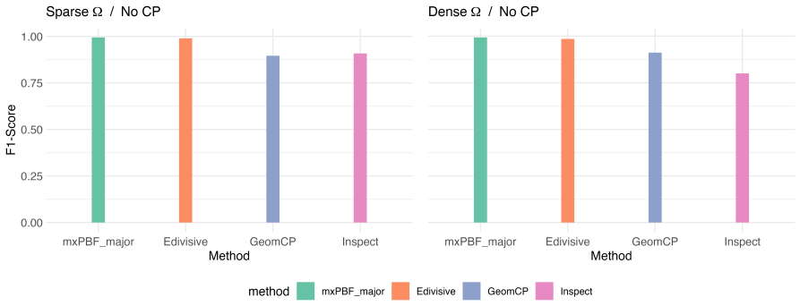
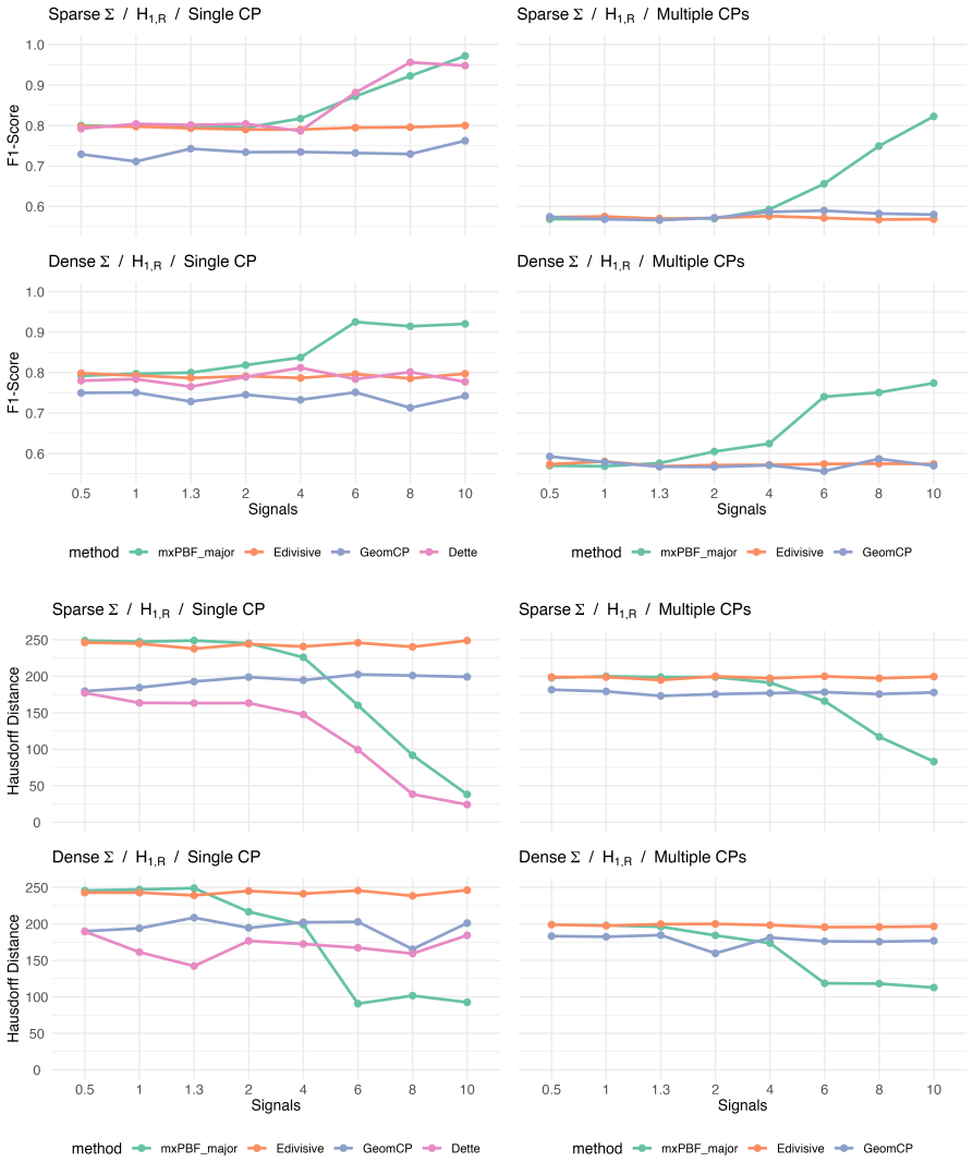
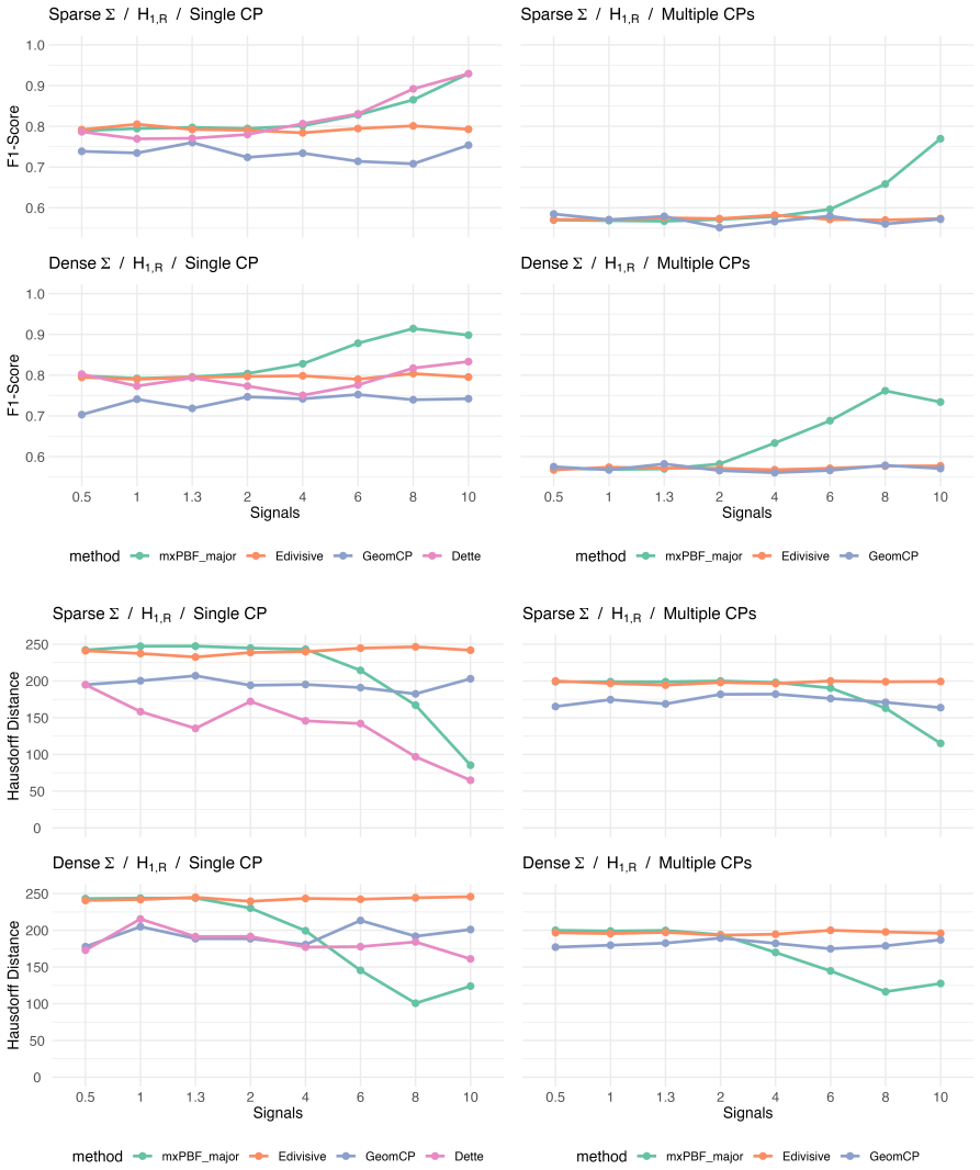
- [Figures 1-6 and Appendix A] Simulation results are reported as point summaries over only 50 datasets without error bars or confidence bands; given the visible variability in F1 scores and Hausdorff distances, reporting variability or replication counts would strengthen the empirical comparisons.
- [Appendix B.1] The word 'controlls' in 'which controlls the empirical false positive rate at 0.05' is a typo; it should be 'controls'.
Circularity Check
No definitional circularity: consistency/localization proofs rely on independent two-sample PBF tail bounds from Lee et al. (2024) and in-text lower-bound constructions; the FPR-based alpha calibration is an unproven applicability gap, not a circular reduction.
full rationale
The load-bearing derivation is not circular. Theorem 2.2 (and 3.2) reduces consistent localization to the per-window mxPBF tail behavior established in Theorem 2.1 (and 3.1); those tail bounds are imported from the previously published two-sample testing analysis in Lee et al. (2024), which does not assume any change point result. The minimax lower bounds (Theorems 2.3, 3.3, 3.4) are proved in the paper by standard Le Cam constructions adapted from Wang and Samworth (2018) and Wang et al. (2021), with citations. The claimed near-optimality is a genuine rate match: when the signal is at the lower-bound threshold psi^2_min asymptotically log(nw or p)/nw, the nw/n upper localization rate is within a log factor of the 1/(n*psi^2_min) lower bound; this is minimax matching, not equivalence-by-definition. The one substantive weakness is a coverage gap, not circularity: Section 4.2 and Appendix B select alpha by FPR calibration using datasets simulated from N_p(mu_hat, Sigma_hat), whereas Theorems 2.1 and 3.1 require a fixed alpha satisfying (7) or alpha > 6*C3, and no result shows the calibrated alpha_hat meets those conditions or that simulation from the pooled sample moments preserves the null distribution when change points exist. Similarly, the multiscale localization claim in Section 4.1 is asserted with 'it can be shown' and no proof. Both are missing-support or robustness issues; neither makes a predicted quantity equal to an input by construction, because the consistency theorems apply to a well-defined fixed-alpha procedure and the calibration is an extra heuristic layered on top of it.
Assumptions & free parameters
free parameters (4)
- alpha (prior concentration exponent) =
selected by FPR calibration; grid 0.01 to 15
- window size nw (or window set N) =
N={25,60,100} in simulations
- threshold Ccp =
10 by default
- covariance prior shape and rate a0, b0, b01, b02 =
0.01
assumptions (5)
- domain assumption Tail probability bounds for the pairwise Bayes factors from Lee et al. (2024) hold as stated.
- domain assumption Data are independent Gaussian draws: N_p(mu_i, Sigma) for the mean case and N_p(0, Sigma_i) for the covariance case.
- domain assumption Window size satisfies (A1) with nw <= n/2 and log(nw or p)/nw = o(1), and for estimation nw <= delta_n.
- ad hoc to paper The FPR calibration simulates a valid null distribution from N_p(muhat, Sigmahat).
- domain assumption The true number of change points K0 is fixed, and the minimum spacing delta_n and signal strength conditions hold.
Cite this review
Pith. "Pith review of Bayesian optimal change point detection in high-dimensions." pith.science (2026). https://pith.science/paper/73H5PI7K
@misc{pith2026241114864,
  author       = {Pith},
  title        = {Pith review of: Bayesian optimal change point detection in high-dimensions},
  year         = {2026},
  howpublished = {\url{https://pith.science/paper/73H5PI7K}},
  note         = {Machine review of arXiv:2411.14864}
}
read the original abstract
We propose the first Bayesian methods for detecting change points in high-dimensional mean and covariance structures. These methods are constructed using pairwise Bayes factors, leveraging modularization to identify significant changes in individual components efficiently. We establish that the proposed methods consistently detect and estimate change points under much milder conditions than existing approaches in the literature. Additionally, we demonstrate that their localization rates are nearly optimal in terms of rates. The practical performance of the proposed methods is evaluated through extensive simulation studies, where they are compared to state-of-the-art techniques. The results show comparable or superior performance across most scenarios. Notably, the methods effectively detect change points whenever signals of sufficient magnitude are present, irrespective of the number of signals. Finally, we apply the proposed methods to genetic and financial datasets, illustrating their practical utility in real-world applications.
Figures


Figures from the paper (22 more)




Reference graph
Works this paper leans on
-
[1]
Avanesov, V. and Buzun, N. (2018). Change-point detection in high-dimensional covariance struc- ture, Electronic Journal of Statistics 12(2): 3254–3294. Berthet, Q. and Rigollet, P. (2013). Optimal detection of sparse principal components in high dimension, The Annals of Statistics 41(4): 1780–1815. Bleakley, K. and Vert, J.-P. (2011). The group fused las...
arXiv 2018
-
[83]
Yu, B. (1997). Assouad, fano, and le cam, Festschrift for Lucien Le Cam , Springer, pp. 423–435. Zhang, N. R. and Siegmund, D. O. (2007). A modified bayes information criterion with applications to the analysis of comparative genomic hybridization data, Biometrics 63(1): 22–32. 56
work page 1997
-
[454]
Enikeeva, F. and Harchaoui, Z. (2019). High-dimensional change-point detection under sparse alternatives, The Annals of Statistics 47(4): 2051–2079. Foret, P. (2019). Sp500r: Easy loading of sp500 stocks data. Github R package version 0.1.0. Fryzlewicz, P. (2014). Wild binary segmentation for multiple change-point detection, The Annals of Statistics 42(6)...
work page 2019
-
[507]
Van den Burg, G. J. and Williams, C. K. (2020). An evaluation of change point detection algorithms, arXiv preprint arXiv:2003.06222 . Vostrikova, L. J. (1981). Detecting “disorder” in multidimensional random processes., Soviet Math- ematics Doklady 24: 55–59. Wang, D., Yu, Y. and Rinaldo, A. (2021). Optimal covariance change point localization in high dim...
arXiv 2020
-
[4419]
Lee, K., You, K. and Lin, L. (2024). Bayesian optimal two-sample tests for high-dimensional gaussian populations, Bayesian Analysis 19(3): 869–893. Matteson, D. S. and James, N. A. (2014). A nonparametric approach for multiple change point analysis of multivariate data, Journal of the American Statistical Association 109(505): 334–345. 55 Pollard, D. (200...
work page 2024
Reviewed August 12, 2026 · model on record in the stance chip above.
Discussion (0). Continue with ORCID to comment.