REVIEW 3 major objections 5 minor 30 references
FieldTNN-based machine learning method for Maxwell eigenvalue problems
T0 review · 3 major / 5 minor · reviewed 2026-08-12 · deepseek-v4-flash
Pith's one-line read FieldTNN solves Maxwell eigenvalue problems in tensor and non-tensor cavities, with spurious modes filtered automatically by a divergence-free penalty in the loss.
desk verdict Impressive numerics for Maxwell eigenvalues with FieldTNN, but the divergence-free filter's justification doesn't match the paper's own norm definitions. read the letter →
The pith
A machine-rendered reading of the paper's core claim, the machinery that carries it, and where it could break.
The reading
What carries the argument
The central object is the FieldTNN itself: a rank-$p$ vector function $\Psi(x;\Theta) = \sum_{k=1}^p u_k \hat\Psi_k(x;\Theta)$, where each vector-valued rank-one block $\hat\Psi_k$ has components that are products of one-dimensional subnetworks, one subnetwork per coordinate per field component. This product structure lets the curl and divergence of the network be written as sums of products of one-dimensional functions, so the stiffness and mass matrices $S_{ji}=A(\hat\Phi_i,\hat\Phi_j)$ and $M_{ji}=B(\hat\Phi_i,\hat\Phi_j)$ of the Galerkin discretization factor into one-dimensional integrals and are assembled by high-order one-dimensional quadrature in $O(d^3 M N)$ operations. The machinery that carries the spurious-mode filtering argument is the ratio $\rho = |E_{NN}|^2_{H(\mathrm{div};\Omega)}/|E_{NN}|^2_{H(\mathrm{curl};\Omega)}$ added as a penalty in the loss (5.13). For non-tensor domains, the paper constructs compactly supported subnetworks by composing each subnetwork with the one-dimensional clamping function $g_{[a,b]}(x)$ built from ReLU units, so that basis functions vanish outside their subdomain and global matrices are assembled by summing subdomain contributions. The boundary condition $E\times n=0$ is enforced by multiplying each field component by analytic factors $\gamma_i(x_i)$ that vanish on the appropriate faces.
What would settle it
A concrete test: construct a Maxwell eigenvalue problem whose relaxed variational form (2.2) has a multiple spurious eigenvalue, or seed the FieldTNN ansatz with two linearly independent curl-free vector fields of equal Rayleigh quotient, and train with loss (5.13). If any reported eigenpair has a large curl-free component yet still attains a small loss and a small ratio $\rho$, the filter has misclassified it; the paper provides no theoretical or numerical evidence for this degenerate case.
Extended reading notes
Core claim
The paper's central claim is that a FieldTNN—a vector-valued tensor neural network in which each component of the field is a sum of products of one-dimensional subnetworks—can approximate Maxwell eigenpairs to high accuracy while automatically excluding spurious ones. The key mechanism is a loss function $L_{\mathrm{Maxwell}}(\lambda_{k,NN}, E_{k,NN}) = \lambda_{k,NN} + \beta |E_{k,NN}|^2_{H(\mathrm{div};\Omega)} / |E_{k,NN}|^2_{H(\mathrm{curl};\Omega)}$ applied to the leading generalized eigenpairs of the FieldTNN Galerkin system. Because genuine eigenfunctions are divergence-free, their $H(\mathrm{div})$ norm is small, while spurious eigenpairs of the relaxed variational formulation are curl-free when simple, making their $H(\mathrm{curl})$ norm small and the ratio large. Minimizing the summed loss therefore drives the network toward divergence-free eigenspaces, and the paper's numerical experiments show no spurious eigenvalues surviving. On tensor domains the basis functions are products of subnetworks over coordinate intervals; on non-tensor domains the domain is split into tensor subdomains and locally supported subnetworks are trained in each, mimicking spectral element assembly. The paper claims this is the first application of tensor neural networks to vector field eigenvalue problems and the first extension of the TNN framework to non-tensor computational domains.
Load-bearing premise
The method's ability to throw out fake solutions depends on a clean split: true eigen-solutions carry no divergence, while simple fake solutions carry no curl, so the ratio in the loss separates them; if a fake eigenvalue is repeated or mixed with a real one, that split is no longer guaranteed and the paper gives no analysis for that case.
Editorial extensions
If this is right
- Leading Maxwell eigenvalues in smooth 2D and 3D cavities can be computed with relative errors around $10^{-9}$ to $10^{-8}$, competitive with or better than the two-grid edge-element and mixed spectral element comparisons in the paper.
- Spurious eigenpairs are filtered during training rather than in a separate post-processing pass, so the output eigenpairs satisfy the divergence-free condition to the tolerance shown by small $|E_{NN}|_{H(\mathrm{div};\Omega)}$ values.
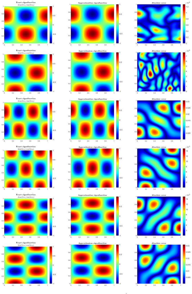
- The method applies to non-tensor domains such as 2D and 3D L-shaped cavities, where singular eigenfunctions with unbounded gradients are still captured, with largest relative eigenvalue errors around $10^{-3}$ for the singular leading mode.
- The same FieldTNN construction is claimed to extend to other vector field equations—Maxwell equations, Stokes equations, magnetohydrodynamics—since the architecture and quadrature splitting depend only on the product structure of the field components.
- Because integration is reduced to one-dimensional quadrature with polynomial complexity in dimension, the approach avoids the curse of dimensionality for the variational forms used here.
Reading between the lines
- Editorial inference: The divergence-free filter relies on the sharp distinction between divergence-free real modes and curl-free simple spurious modes; if a spurious eigenvalue is multiple or nearly degenerate, the ratio $\rho$ may not separate eigenpairs, and the method would need a stabilizer or deflation to stay reliable.
- Editorial inference: The penalty parameter $\beta$ creates a trade-off: too small leaves spurious modes with small loss, too large distorts the eigenvalue estimate; a principled schedule for $\beta$ is a natural next test.
- Editorial inference: One could test the method on a domain with a reentrant corner of different angle, where the singular exponent of the Maxwell eigenfunction changes, to see whether the reported accuracy on the 90-degree L-shape degrades.
- Editorial inference: Because the boundary condition is enforced by analytic multipliers rather than by the network itself, the method's extension to curved or material-interface boundaries would require rederiving those multipliers, which is a concrete limitation not addressed in the paper.
Editorial analysis
A structured set of objections, weighed in public.
Referee Report
Summary. The paper introduces FieldTNN, a tensor neural network architecture for vector-valued functions, and applies it to the Maxwell eigenvalue problem in two and three dimensions on both tensor-product and non-tensor domains. For non-tensor domains, the method uses locally compactly supported FieldTNN bases on subdomains. The authors propose a loss function that adds a penalty proportional to a H(div)/H(curl) ratio of the computed eigenfunctions in order to automatically filter spurious, non-divergence-free eigenpairs. Numerical experiments on square, L-shaped, inhomogeneous, cubic, and 3D L-shaped cavities report very high accuracy for tensor domains and moderate accuracy for singular non-tensor domains, with comparisons to existing finite element and spectral element results.
Significance. If the claims are substantiated, this is a useful extension of the TNN framework to vector field eigenvalue problems and to non-tensor computational domains. The reported tensor-domain accuracy is genuinely strong: relative eigenvalue errors around 1e-8 to 1e-9 in the square and cube cavities, competitive with or better than the cited standard methods, and the quadrature splitting in Section 5.1 provides a concrete complexity argument for avoiding tensor-product quadrature in low-rank formats. The treatment of non-tensor domains through locally supported TNN bases is a reasonable and potentially transferable idea. However, the central claim that spurious eigenpairs are automatically filtered by the proposed ratio-based penalty is not established as written; the mathematical justification in Section 5.2.1 is inconsistent with the norms defined in Section 2 and does not cover the reported numerical evidence.
major comments (3)
- [Section 5.2.1, Eq. (5.13), Tables 6.1, 6.3, 6.5, 6.7, 6.9] The filter ratio as written is incompatible with the norms defined in Section 2. With the full H(div) and H(curl) norms, a normalized real eigenpair satisfies rho = ||E||^2_H(div)/||E||^2_H(curl) = (1 + ||div E||^2)/(1 + ||curl E||^2) = 1/(1 + lambda), which is not close to zero for small eigenvalues; for the first square-cavity mode lambda = pi^2 this gives approximately 0.092. Yet the tables report |E_NN|_H(div) around 1e-9 for normalized eigenfunctions, which is impossible under that same norm because the L2 component alone is of order 1. The text must mean the seminorm ||div E||_L2, not the H(div) norm. This needs to be stated explicitly and consistently throughout, and the separation mechanism must be re-derived for the seminorm, since the claim that the numerator approaches zero is otherwise false.
- [Section 5.2.1, Section 2] The justification for separating spurious from real eigenpairs is incomplete. The cited curl-free property is stated only for simple spurious eigenvalues, and the argument that the denominator of the ratio approaches zero relies on that property. For multiple or near-degenerate spurious eigenvalues, no analysis is provided, and a curl-free field can have arbitrarily small divergence, so the ratio with the seminorm does not guarantee a large value for all spurious modes. Since the paper's advertised mechanism is 'automatic filtering of spurious eigenpairs', the authors should either prove the separation under the intended seminorm, or provide a numerical study covering clustered and multiple spurious eigenvalues.
- [Sections 5.3 and 6, Eq. (5.13)] The penalty parameter beta in the loss function (5.13) is never disclosed, and the text does not explain how beta is chosen or how the penalty interacts with the generalized eigenvalue problem solved in post-processing. The final eigenvalues are extracted from the GEVP (5.4), not directly from the minimized loss, so it is unclear whether the penalty term actually changes the eigenfunction basis during training or merely adds a constant that vanishes for divergence-free fields. The authors should report beta for each numerical example, discuss its influence on the computed eigenvalues and on the reported H(div) values, and ideally give an error or consistency analysis showing that the penalty does not bias the converged eigenpairs.
minor comments (5)
- [Sections 6.1, 6.3] The name is misspelled as 'FiedTNN' in the text introducing the numerical results; it should be 'FieldTNN'.
- [Algorithm 2, Section 5.3] Algorithm 2 has two steps labeled 'Step 1'; the second one should be renumbered.
- [Section 5.2.1] The word 'filter' is misspelled as 'fileter' in 'fileter ratio'.
- [Figure 3.2 caption] The caption contains the typo 'pruple', which should be 'purple'.
- [Section 6.2] The numerical setup for the 2D L-shaped cavity reports only Adam optimization, whereas Sections 6.1 and 6.4 describe an additional L-BFGS refinement phase; it would be helpful to state whether such refinement was used or omitted for consistency.
Circularity Check
No significant circularity: the FieldTNN Maxwell eigenvalues are outputs of a generalized eigenproblem benchmarked against independent references, and the prior TNN citations are background, not load-bearing.
full rationale
The paper's derivation chain is self-contained with respect to its central numerical claim. The approximate eigenvalues are obtained by assembling stiffness and mass matrices from FieldTNN basis functions and solving the generalized eigenproblem SU = lambda_NN M U (Eq. (5.4), with entries (5.10)-(5.11)); they are not fitted constants renamed as predictions. The loss function (5.13) is a sum of Rayleigh quotients plus a divergence-free penalty, but the penalty does not define the eigenvalues by construction; it only shapes the trial space during training, and the final eigenpairs are extracted from the generalized eigenproblem. The paper compares against independent benchmarks and prior numerical methods: exact eigenvalues for square and cube cavities, Dauge's benchmark for L-shaped cavities, and published FEM/mixed spectral element results. Citations to earlier TNN works by the same authors ([27]-[29]) supply architecture and quadrature background, but the Maxwell extension and the non-tensor domain construction are built explicitly in this paper through Eqs. (4.1)-(4.7) and (5.14), so the central contribution does not reduce to those citations. The cited curl-free property of simple spurious eigenpairs comes from external sources ([5], [13]), not from the authors' own prior work. One internal issue is noted but is not circularity: the filtering argument in Section 5.2.1 states that for divergence-free real eigenpairs the numerator of the ratio |E|^2_H(div)/|E|^2_H(curl) 'will approach to 0', and Tables 6.1, 6.3, 6.5, 6.7, 6.9 report |E_NN|_H(div) values near 1e-9. Under the H(div) norm defined in Section 2, which includes the L2 term, a normalized divergence-free field has |E|_H(div) = |E|_L2 = 1, not ~0; the tables are consistent only if a divergence seminorm is intended. This is a correctness or reporting inconsistency about the filtering mechanism, not a case where an output is equal to an input by definition. Therefore no circular step is exhibited, and the appropriate score is 0.
Assumptions & free parameters
free parameters (5)
- rank p =
50 or 100 depending on example
- penalty parameter beta =
not reported
- network architecture (hidden layers and neurons) =
3 hidden layers with 50 or 100 neurons
- training schedule (learning rate, epochs, optimizer) =
varies per example
- quadrature points per dimension =
800 or 1600
assumptions (4)
- standard math The variational form (2.2) and the min-max principle justify using the sum of the first M Rayleigh quotients as a loss function.
- ad hoc to paper Simple spurious eigenpairs of the relaxed form (2.2) are curl-free, so the ratio |E|_H(div)^2/|E|_H(curl)^2 separates them from real eigenpairs.
- ad hoc to paper Gradient descent on the non-convex loss (5.13) converges to the leading M eigenpairs of the FieldTNN Galerkin problem.
- ad hoc to paper FieldTNN bases with local compact support can approximate singular Maxwell eigenfunctions (e.g., r^{-1/3} behavior at reentrant corners) to the reported accuracy.
Cite this review
Pith. "Pith review of FieldTNN-based machine learning method for Maxwell eigenvalue problems." pith.science (2026). https://pith.science/paper/WRJHXYPV
@misc{pith2026241115828,
  author       = {Pith},
  title        = {Pith review of: FieldTNN-based machine learning method for Maxwell eigenvalue problems},
  year         = {2026},
  howpublished = {\url{https://pith.science/paper/WRJHXYPV}},
  note         = {Machine review of arXiv:2411.15828}
}
read the original abstract
The aim of this paper is to introduce a FieldTNN-based machine learning method for solving the Maxwell eigenvalue problem in both 2D and 3D domains, including both tensor and non-tensor computational regions. First, we extend the existing TNN-based approach to address the Maxwell eigenvalue problem, a fundamental challenge in electromagnetic field theory. Second, we tackle non-tensor computational domains, which represents a novel and significant contribution of this work. Third, we incorporate the divergence-free condition into the optimization process, allowing for the automatic filtering of spurious eigenpairs. Numerical examples are presented to demonstrate the efficiency and accuracy of our algorithm, underscoring its potential for broader applications in computational electromagnetics.
Figures


Figures from the paper (6 more)



Reference graph
Works this paper leans on
- [1]
-
[2]
I. Babu s ka and J. Osborn. Eigenvalue problems. In Finite Element Methods (Part 1) , volume 2 of Handbook of Numerical Analysis , pages 641--787. Elsevier, 1991
work page 1991
- [3]
-
[4]
J. Conway. A course in functional analysis . Springer, Berlin, 2007
work page 2007
-
[5]
M. Costabel and M. Dauge. Computation of resonance frequencies for Maxwell equations in non-smooth domains , pages 125--161. Springer, Berlin, Heidelberg, 2003
work page 2003
-
[6]
M. Dauge. https://perso.univrennes1.fr/monique.dauge/core/index.html
- [7]
-
[8]
W. E and B. Yu. The D eep R itz M ethod: A deep learning-based numerical algorithm for solving variational problems. Communications in Mathematics and Statistics , 6(1):1--12, 2018
work page 2018
Show all 30 references
-
[9]
Gastaldi
L. Gastaldi. F. Bertrand, D. Boffi. Approximation of the M axwell eigenvalue problem in a least-squares setting. Computers & Mathematics with Applications. , 148:302--312, 2023
2023
-
[10]
J. Han, J. Lu, and M. Zhou. Solving high-dimensional eigenvalue problems using deep neural networks: A diffusion monte carlo like approach. Journal of Computational Physics , 423:109792, 2020
2020
-
[11]
Hiptmair
R. Hiptmair. Finite elements in computational electromagnetism. Acta Numerica , 11:237–339, 2002
2002
-
[12]
Jiang and J
J. Jiang and J. An. Numerical approximation based on a decoupled dimensionality reduction scheme for M axwell eigenvalue problem. Mathematical Methods in the Applied Sciences , 46(16):17367--17387, 2023
2023
-
[13]
Ciarlet Jr and G
P. Ciarlet Jr and G. Hechme. Computing electromagnetic eigenmodes with continuous galerkin approximations. Computer Methods in Applied Mechanics and Engineering , 198(2):358--365, 2008
2008
-
[14]
Kwan and J
Y.-Y. Kwan and J. Shen. An efficient direct parallel spectral-element solver for separable elliptic problems. Journal of Computational Physics , 225(2):1721--1735, 2007
2007
-
[15]
Lagaris, A
I.E. Lagaris, A. Likas, and D.I. Fotiadis. Artificial neural network methods in quantum mechanics. Computer Physics Communications , 104(1):1--14, 1997
1997
-
[16]
H. Li, Q. Zhai, and J. Chen. Neural-network-based multistate solver for a static schr\" o dinger equation. Physical Review A , 103:032405, 2021
2021
-
[17]
Y. Li, Z. Lin, Y. Wang, and H. Xie. Tensor neural network interpolation and its applications. arXiv:2404.07805 , 2024
2024 arXiv
-
[18]
Z. Li, Z. Qiao, and T. Tang. Numerical solution of differential equations: introduction to finite difference and finite element methods . Cambridge University Press, Cambridge, 2017
2017
-
[19]
N. Liu, Y. Tang, X. Zhu, L. Tobón, and Q. Liu. Higher-order mixed spectral element method for M axwell eigenvalue problem. In 2013 IEEE Antennas and Propagation Society International Symposium (APSURSI) , pages 1646--1647, 2013
2013
-
[20]
N. Liu, L. Tobón, Y. Tang, and Q. Liu. Mixed spectral element method for 2 D M axwell’s eigenvalue problem. Communications in Computational Physics , 17(2):458–486, 2015
2015
-
[21]
N. Liu, L. Tobón, Y. Zhao, Y. Tang, and Q. Liu. Mixed spectral-element method for 3- D maxwell's eigenvalue problem. IEEE Transactions on Microwave Theory and Techniques , 63(2):317--325, 2015
2015
-
[22]
P. Monk. Finite Element Methods for Maxwell's Equations . Oxford University Press, 2003
2003
-
[23]
Paszke, S
A. Paszke, S. Gross, S. Chintala, G. Chanan, E. Yang, Z. DeVito, Z. Lin, A. Desmaison, L. Antiga, and A. Lerer. Automatic differentiation in P y T orch. In NIPS 2017 Workshop on Autodiff , 2017
2017
-
[24]
Y. Saad. Numerical Methods For Large Eigenvalue Problems . Society for Industrial and Applied Mathematics, 2011
2011
-
[25]
J. Shen, T. Tang, and L.-L. Wang. Spectral methods: algorithms, analysis and applications , volume 41. Springer Science & Business Media, 2011
2011
-
[26]
Sun and A
J. Sun and A. Zhou. Finite Element Methods for Eigenvalue Problems . Chapman and Hall/CRC, 1st edition, 2016
2016
-
[27]
Y. Wang, P. Jin, and H. Xie. Tensor neural network and its numerical integration. Journal of Computational Mathematics , 42(6):1714--1742, 2024
2024
-
[28]
Y. Wang, Z. Lin, Y. Liao, H. Liu, and H. Xie. Solving high dimensional partial differential equations using tensor neural network and a posteriori error estimators. Journal of Scientific Computing , 101:67, 2024
2024
-
[29]
Wang and H
Y. Wang and H. Xie. Computing multi-eigenpairs of high-dimensional eigenvalue problems using tensor neural networks. Journal of Computational Physics , 506:112928, 2024
2024
-
[30]
J. Zhou, X. Hu, L. Zhong, S. Shu, and L. Chen. Two-grid methods for M axwell eigenvalue problems. SIAM Journal on Numerical Analysis , 52(4):2027--2047, 2014
2027
Reviewed August 12, 2026 · model on record in the stance chip above.
Discussion (0). Continue with ORCID to comment.