REVIEW 3 major objections 5 minor 49 references
Runge-Kutta Discontinuous Galerkin Method Based on Flux Vector Splitting with Constrained Optimization-based TVB(D)-minmod Limiter for Solving Hyperbolic Conservation Laws
T0 review · 3 major / 5 minor · reviewed 2026-08-12 · deepseek-v4-flash
Pith's one-line read This paper brings flux vector splitting into the discontinuous Galerkin framework and adds a constrained-optimization TVB minmod limiter that keeps high-order accuracy while suppressing oscillations near shocks.
desk verdict A novel constrained-optimization limiter that deserves referee time, but the paper's quantitative evidence is unreliable and the weight-dependence undercuts its central claim. read the letter →
The pith
A machine-rendered reading of the paper's core claim, the machinery that carries it, and where it could break.
The reading
What carries the argument
The carrying object is the split flux identity $F = F^+ + F^-$, used both to build the DG numerical flux and to motivate the limiter's optimization. In one dimension the numerical flux at an interface is $\hat{F}_{i+1/2} = \hat{F}^+_{i+1/2} + \hat{F}^-_{i+1/2}$, with $\hat{F}^+$ taken from the left state and $\hat{F}^-$ from the right state; in two dimensions the same splitting is applied to the normal flux. The limiter's machinery is a linear weighted-sum objective whose smoothness term is the WENO smoothness indicator (a scaled sum of squared derivatives), rewritten as a positive-semidefinite quadratic form in the modal coefficients, while the $L^2$ term is a diagonal quadratic form measuring distance to the original high-order solution. Lagrange multipliers enforce the minmod-modified boundary constraints, producing a small saddle-point linear system to solve per troubled cell. The interpolation-based characteristic transformation instead applies the left eigenvector matrix $L$ to sampled point values rather than to modal coefficient columns, and the paper proves this coincides with the moment transformation when all components share identical basis functions.
What would settle it
Fix the weights once, say $\omega_{\mathrm{IS}}=0.75$, $\omega_{L^2}=0.25$, and run the limiter on the paper's own $P^3$ Burgers shock test, the $P^3$ Sod problem, and the $P^5$ Shu-Osher problem; if any of those runs shows visible overshoot, a loss of the $(K+1)$-order convergence rate on smooth parts, or a divergence, then the claimed balance depends on per-problem tuning rather than on the method itself.
Extended reading notes
Core claim
On its own terms, the paper claims two new things. First, the FVS method—splitting the flux $F$ into $F^+$ and $F^-$ by Jacobian eigenvalue splitting or by Mach-number splitting, then applying upwind numerical sub-fluxes—has been incorporated for the first time into the DG weak formulation; the resulting FVS-DG scheme empirically delivers $(K+1)$-th order convergence for $P^K$ approximations on scalar and system equations in one and two dimensions. Second, the classical TVB(D)-minmod limiter, which gives only two correction conditions in 1D and four in 2D and therefore cannot determine all modal coefficients of high-order polynomials, is made well-posed by solving a constrained optimization problem: minimize $w_{\mathrm{IS}}\,\mathrm{IS}(u^{\mathrm{mod}}) + w_{L^2}\|u^{\mathrm{mod}} - u^{\mathrm{old}}\|_{L^2}$ subject to the cell average and the minmod-corrected boundary values. The paper further proposes an interpolation-based characteristic transformation that it proves equivalent to the moment characteristic transformation in 1D when all components share the same basis, and derives a Steger-Warming numerical flux for scalar equations from the Jacobian-FVS perspective.
Load-bearing premise
The limiter's promised balance between accuracy and oscillation control rests on the user picking the two weights in the optimization objective well; the paper changes those weights from test to test and gives no automatic rule for choosing them.
Editorial extensions
If this is right
- If FVS-DG is correct, DG users can replace Lax-Friedrichs or Riemann-solver fluxes with Steger-Warming, van Leer, or AUSM split fluxes and still observe optimal $(K+1)$-order convergence, while inheriting the lower dissipation of FVS.
- If the IS-$L^2$-TVB(D)-minmod limiter performs as claimed, the standard TVB(D)-minmod limiter can be extended to $P^K$ approximations for any $K$ by solving a small linear system per troubled cell, with the smoothness term preventing Gibbs oscillations and the $L^2$ term protecting accuracy.
- The interpolation-based characteristic transformation gives an equivalent but simpler route to local characteristic decomposition in DG when all components share basis functions, and the paper's local-freezing proposal uses edge integral averages rather than cell averages.
- The scalar Steger-Warming flux, proved consistent, Lipschitz, and monotone for linear advection and Burgers' equation, makes the DG scheme satisfy a cell entropy inequality and $L^2$ stability for those equations, with slightly lower dissipation than Lax-Friedrichs in the paper's long-time tests.
- Numerical experiments on Sod, Lax, Shu-Osher, Blast, and two-dimensional Riemann problems indicate that $P^3$ and $P^5$ approximations with the new limiter capture discontinuities without visible overshoot on the tested meshes.
Reading between the lines
- A testable extension would replace the user-chosen weights with a local heuristic, for example setting $\omega_{\mathrm{IS}}$ high when a troubled-cell indicator flags a strong discontinuity and lowering it in mildly oscillatory regions; the paper gives no such rule.
- The FVS-DG construction should transfer to other hyperbolic systems that admit homogeneous-flux or Mach-number splitting, such as magnetohydrodynamics, but the paper only demonstrates Euler and shallow-water equations; this is an extrapolation.
- Because the equivalence proof for the interpolation-based characteristic transformation assumes all components share the same basis functions, the two transformations could differ for component-dependent bases; the paper leaves that case unexamined.
- A cheaper production variant of the limiter might apply the smoothness-only objective near strong shocks and reserve the $L^2$ term for mild oscillations, since the paper itself notes that the smoothness constraint alone is preferable in extreme shock-tube cases.
Editorial analysis
A structured set of objections, weighed in public.
Referee Report
Summary. The paper proposes a Runge-Kutta discontinuous Galerkin (RKDG) method in which the numerical flux is obtained from flux vector splitting (Jacobian-eigenvalue splitting or Mach-number splitting), giving what the authors call FVS-DG in one and two space dimensions. It also introduces a limiter that solves a constrained optimization problem: minimize a weighted combination of the WENO smoothness indicator IS and the L2 deviation from the original high-order solution, subject to the endpoint or boundary-average constraints produced by the TVB(D)-minmod limiter. A separate contribution is an interpolation-based characteristic transformation, with a proof of its equivalence to the moment-based transformation in one dimension when all components share the same basis. The numerical section contains accuracy tests for the Euler and shallow-water systems, scalar and system Riemann problems, and several two-dimensional test cases.
Significance. If the stated claims were fully supported, the paper would offer a simple FVS-type flux for DG and a limiter that can be applied to arbitrary high-order polynomial approximations while controlling oscillations. The derivation of the FVS-DG weak form is transparent, the equivalence proof in Section 7.2 is explicit, and Appendix C contains a useful derivation of a scalar Steger-Warming flux together with proofs of consistency, Lipschitz continuity, and monotonicity. However, the current quantitative support is not sufficient for the main claims: the balancing property of the limiter rests on per-problem tuned weights, and the accuracy tables contain an internal inconsistency. The significance is therefore conditional on a substantial revision of the evidence.
major comments (3)
- [§6.2.3, §8.2–8.3] The central claim that the IS-L2-TVB(D)-minmod limiter balances oscillation suppression and high precision is not established by the evidence presented. The balance is controlled entirely by the user-specified weights omega_IS and omega_L2 in Eqs. (6.28) and (6.34), and these weights are changed from case to case: Example 8.4 uses (1.0, 0.0), Examples 8.7 and 8.10 use (0.75, 0.25), and Examples 8.11 and 8.13–8.15 use (0.8, 0.2). No automatic selection rule, no sensitivity study, and no fixed-weight test across all problems is provided. Moreover, the L2 term pulls the corrected polynomial back toward the original high-order solution, so for larger omega_L2 the limiter can in principle retain the oscillations it is meant to remove. Because the reported runs are tuned per problem, they demonstrate that suitable weights can be found, not that the proposed limiter itself balances the two objectives. Please provide a fixed-weight robustness study and quantitative measures such as overshoot magnitudes and smooth-region L1/L2 errors.
- [Tables 1–4, Example 8.1] The accuracy tables contain an internal inconsistency that prevents verification of the claimed (K+1)-th order accuracy. For the exact solution of Example 8.1, rho*u = -0.7*rho and E = P/(gamma-1) + 0.5*rho*u^2 = 2.5 + 0.245*rho, so the errors of the three conservative variables cannot coincide. Nevertheless, Tables 1–4 report exactly the same L2 and L1 errors for rho, rho*u, and E; for instance Table 1 lists the L2-error 2.4737E-04 for all three variables at Mesh 10. This indicates either copy-paste errors or a defect in the error computation. Please provide corrected per-component errors and convergence orders for both the AUSM and Steger-Warming FVS-DG runs.
- [§1 and §4] The sentence that 'The FVS method inherently does not introduce any error' is not correct as stated. Flux splitting at the continuous PDE level is exact, but the discretized FVS-DG flux, e.g. hat-F_{i+1/2} = F^+(U^L_{i+1/2}) + F^-(U^R_{i+1/2}) in Eq. (4.9), is an approximate upwind numerical flux and introduces numerical dissipation, as the discussion of S-W versus L-F splitting in Appendix C itself indicates. The paper should remove or qualify this claim; otherwise the accuracy discussion is based on a false premise about the numerical flux.
minor comments (5)
- [Throughout] There are numerous typos, including 'Numderical' (Example 8.1 and elsewhere), 'uniquely spaced' (Figure 1 caption and throughout), 'T VB' and 'Minmd' in Section 6, and 'setp4' in Section 7; these should be corrected in a revision.
- [§6.2.3] The weights are described as forming a convex combination, but the condition omega_IS + omega_L2 = 1 is never stated; please state the admissible range explicitly.
- [§7.2] Proposition 7.1 should explicitly assume that the interpolation points are distinct so that the matrices P^{(i)} in Eq. (7.14) are invertible; currently this assumption is implicit.
- [§4] The derivation in Section 4 eventually reduces to the standard DG weak form with a single numerical flux hat-F = hat-F^+ + hat-F^- (Eqs. (4.7)–(4.8)); the novelty discussion would be clearer if this reduction were stated explicitly rather than presenting the two sub-fluxes as a separate formulation.
- [§8.2] The claims about overshoot and smoothness in Examples 8.4–8.6 are based only on visual inspection of plots; adding quantitative overshoot values or error norms would make the comparisons reproducible.
Circularity Check
No significant circularity: the FVS-DG and limiter constructions are self-contained and validated against independent exact solutions.
full rationale
I walked the derivation chain. The FVS-DG scheme is obtained by splitting F into F+ and F- (Section 4), which is an exact identity, and then applying integration by parts; the upwind choice F^± = F^±(U_(L/R)) is a design decision, not a fitted input. The IS-L2-TVB(D)-minmod limiter (Eqs. 6.28-6.34) is a constrained optimization whose objective explicitly includes both the smoothness indicator IS and the L2 distance to the unfiltered solution; this is the construction itself, and the paper's claim of balancing oscillation suppression and accuracy is checked against independent exact solutions in Section 8 rather than being derived from the objective alone. Proposition 7.1 proves, under the stated assumption of identical basis functions, that interpolation-based and moment characteristic transformations coincide; the proof is algebraic and self-contained, so no circularity is involved. The load-bearing cited results ([1], [42], etc.) are not by the present author, so there is no self-citation chain. I note two non-circular weaknesses: the convergence tables for Example 8.1 report identical L2/L1 errors for rho, rho*u, and E even though the exact solution has constant u=-0.7 and P=1, which is arithmetically inconsistent and weakens the accuracy evidence; and the limiter weights omega_IS, omega_L2 are changed from example to example without an automatic selection rule, which is a robustness concern. Neither weakness makes the derivation circular.
Assumptions & free parameters
free parameters (2)
- omega_IS and omega_L2 weights =
varies: (1.0, 0.0), (0.75, 0.25), (0.8, 0.2)
- TVB parameter M =
1.0
assumptions (4)
- domain assumption The flux function F(U) admits an exact flux vector splitting F=F+ + F- with positive and negative parts based on local eigenvalues or Mach number.
- domain assumption The numerical flux formed from one-sided split fluxes is consistent and produces a stable DG discretization.
- ad hoc to paper The constrained optimization problem has a unique solution and its KKT system (6.18)-(6.19) is nonsingular for every polynomial degree and mesh configuration.
- ad hoc to paper Bi-objective weights can balance oscillation suppression and accuracy.
Cite this review
Pith. "Pith review of Runge-Kutta Discontinuous Galerkin Method Based on Flux Vector Splitting with Constrained Optimization-based TVB(D)-minmod Limiter for Solving Hyperbolic Conservation Laws." pith.science (2026). https://pith.science/paper/WUKFNKE3
@misc{pith2026241116367,
  author       = {Pith},
  title        = {Pith review of: Runge-Kutta Discontinuous Galerkin Method Based on Flux Vector Splitting with Constrained Optimization-based TVB(D)-minmod Limiter for Solving Hyperbolic Conservation Laws},
  year         = {2026},
  howpublished = {\url{https://pith.science/paper/WUKFNKE3}},
  note         = {Machine review of arXiv:2411.16367}
}
read the original abstract
The flux vector splitting (FVS) method has firstly been incorporated into the discontinuous Galerkin (DG) framework for reconstructing the numerical fluxes required for the spatial semi-discrete formulation, setting it apart from the conventional DG approaches that typically utilize the Lax-Friedrichs flux scheme or classical Riemann solvers. The control equations of hyperbolic conservation systems are initially reformulated into a flux-split form. Subsequently, a variational approach is applied to this flux-split form, from which a DG spatial semi-discrete scheme based on FVS is derived. In order to suppress numerical pseudo-oscillations, the smoothness measurement function IS from the WENO limiter is integrated into the TVB(D)-minmod limiter, constructing an optimization problem based on the smoothness factor constraint, thereby realizing a TVB(D)-minmod limiter applicable to arbitrary high-order polynomial approximation. Subsequently, drawing on the ``reconstructed polynomial and the original high-order scheme's L2 -error constraint'' from the literature [1] , combined with our smoothness factor constraint, a bi-objective optimization problem is formulated to enable the TVB(D)-minmod limiter to balance oscillation suppression and high precision. As for hyperbolic conservation systems, limiters are typically required to be used in conjunction with local characteristic decomposition. To transform polynomials from the physical space to the characteristic space, an interpolation-based characteristic transformation scheme has been proposed, and its equivalence with the original moment characteristic transformation has been demonstrated in one-dimensional scenarios. Finally, the concept of ``flux vector splitting based on Jacobian eigenvalue decomposition'' has been applied to the conservative linear scalar transport equations and the nonlinear Burgers' equation.
Figures
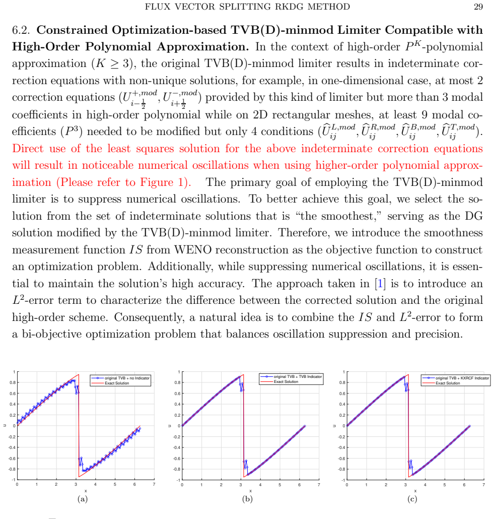


Figures from the paper (17 more)


Reference graph
Works this paper leans on
-
[1]
New two-dimensional slope limit ers for discontinuous Galerkin methods on arbitrary meshes [J]
HOTEIT H, ACKERER P, MOSE R, et al. New two-dimensional slope limit ers for discontinuous Galerkin methods on arbitrary meshes [J]. International Journal f or Numerical Methods in Engineering, 2004, 61: 2566-93. (document), 1, 6.2, 6.2.3, 6.2.3
work page 2004
-
[2]
Hyperbolic Conservation Laws in Continuum Physics [M]
DAFERMOS C M. Hyperbolic Conservation Laws in Continuum Physics [M]. 4th ed. Springer. 2016: XII Introduction. 1
work page 2016
-
[3]
V AN LEER B. Flux-vector splitting for the Euler equations; proce edings of the Eighth International Conference on Numerical Methods in Fluid Dynamics: Proceedings of the Conference, Rheinisch- Westf¨ alische Technische Hochschule Aachen, Germany, June 28– July 2, 1982, F, 2005 [C]. Springer. 1, 3.2.1
work page 1982
-
[4]
V AN LEER B, THOMAS J L, ROE P L, et al. A comparison of numerical fl ux formulas for the Euler and Navier-Stokes equations; proceedings of the 8th AIAA Compu tational Fluid Dynamics Conference, 1987 [C]. 1
work page 1987
-
[5]
STEGER J L, W ARMING R. Flux vector splitting of the inviscid gasdyn amic equations with application to finite-difference methods [J]. Journal of computational physics , 1981, 40(2): 263-93. 1
work page 1981
-
[6]
BERM´ uDEZ A, V´ aZQUEZ M. Flux-vector and flux-difference splitting methods for the shallow water equations in a domain with variable depth [M]. Computer Modelling of Seas and Coastal Regions. Springer. 1992: 255-67. 1, B.1.2, B.2.2
work page 1992
-
[7]
LIOU M-S. Ten years in the making-AUSM-family; proceedings of t he 15th AIAA Computational Fluid Dynamics Conference, F, 2001 [C]. 1
work page 2001
-
[8]
Triangular mesh methods for the neutron tra nsport equation [Z]
REED W H, HILL T R. Triangular mesh methods for the neutron tra nsport equation [Z]. Conference: National topical meeting on mathematical models and computationa l techniques for analysis of nuclear systems, Ann Arbor, Michigan, USA, 8 Apr 1973; Other Informatio n: Orig Receipt Date: 31-DEC-73. United States. 1973: Medium: ED; Size: Pages: 23 1
work page 1973
Show all 49 references
-
[9]
The Local Discontinuous Galerkin Method f or Time-Dependent Convection- Diffusion Systems [J]
COCKBURN B, SHU C-W. The Local Discontinuous Galerkin Method f or Time-Dependent Convection- Diffusion Systems [J]. SIAM Journal on Numerical Analysis, 1998, 35: 2440-63. 1
1998
-
[10]
A direct discontinuous Galerkin method for the generalized Korteweg–de Vries equation: Energy conservation and boundary effect [J]
YI N, HUANG Y, LIU H. A direct discontinuous Galerkin method for the generalized Korteweg–de Vries equation: Energy conservation and boundary effect [J]. Jour nal of Computational Physics, 2013, 242: 351-66. 1
2013
-
[11]
A discontinuous Galerkin finite element method for time dependent partial differential equations with higher order derivatives [J]
CHENG Y, SHU C-W. A discontinuous Galerkin finite element method for time dependent partial differential equations with higher order derivatives [J]. Math Comput , 2008, 77: 699-730. 1
2008
-
[12]
High order semi-Lagrangian discont inuous Galerkin method coupled with Runge-Kutta exponential integrators for nonlinear Vlasov dy namics [J]
CAI X, BOSCARINO S, QIU J. High order semi-Lagrangian discont inuous Galerkin method coupled with Runge-Kutta exponential integrators for nonlinear Vlasov dy namics [J]. Journal of Computational Physics, 2020, 427: 110036. 1
2020
-
[13]
An Eulerian-Lagrangian discontinuous G alerkin method for transport problems and its application to nonlinear dynamics [J]
CAI X, QIU J-M, YANG Y. An Eulerian-Lagrangian discontinuous G alerkin method for transport problems and its application to nonlinear dynamics [J]. Journal of Comp utational Physics, 2021, 439: 110392 1
2021
-
[14]
TVB Runge-Kutta local projection disco ntinuous Galerkin finite element method for conservation laws
COCKBURN B, SHU C-W. TVB Runge-Kutta local projection disco ntinuous Galerkin finite element method for conservation laws. II. General framework [J]. Mathem atics of computation, 1989, 52(186): 411-35. 1 70 ZHENGRONG XIE
1989
-
[15]
TVB Runge-Kutta local projec tion discontinuous Galerkin finite element method for conservation laws III: one-dimensional syste ms [J]
COCKBURN B, LIN S-Y, SHU C-W. TVB Runge-Kutta local projec tion discontinuous Galerkin finite element method for conservation laws III: one-dimensional syste ms [J]. Journal of computational Physics, 1989, 84(1): 90-113. 1
1989
-
[16]
The Runge-Kutta local projectio n discontinuous Galerkin finite element method for conservation laws
COCKBURN B, HOU S, SHU C-W. The Runge-Kutta local projectio n discontinuous Galerkin finite element method for conservation laws. IV. The multidimensional cas e [J]. Mathematics of Computation, 1990, 54(190): 545-81. 1
1990
-
[17]
The Runge-Kutta discontinuous Galerkin method for conservation laws V: multidimensional systems [J]
COCKBURN B, SHU C-W. The Runge-Kutta discontinuous Galerkin method for conservation laws V: multidimensional systems [J]. Journal of computational physics, 19 98, 141(2): 199-224. 1
-
[18]
The Runge-Kutta local projection-disc ontinuous-Galerkin finite element method for scalar conservation laws [J]
COCKBURN B, SHU C-W. The Runge-Kutta local projection-disc ontinuous-Galerkin finite element method for scalar conservation laws [J]. ESAIM: Mathematical Mode lling and Numerical Analysis, 1991, 25(3): 337-61. 1
1991
-
[19]
Parallel, adaptive finite elem ent methods for conservation laws [J]
BISW AS R, DEVINE K D, FLAHERTY J E. Parallel, adaptive finite elem ent methods for conservation laws [J]. Applied Numerical Mathematics, 1994, 14(1-3): 255-83. 1
1994
-
[20]
An adaptive discont inuous Galerkin technique with an orthogonal basis applied to compressible flow problems [J]
REMACLE J-F, FLAHERTY J E, SHEPHARD M S. An adaptive discont inuous Galerkin technique with an orthogonal basis applied to compressible flow problems [J]. SIA M review, 2003, 45(1): 53-72. 1
2003
-
[21]
Point-wise and cell average error estimates of the DG and LDG methods for 1D hyperbolic and parabolic equations [J]
CAO W, ZHANG Z. Point-wise and cell average error estimates of the DG and LDG methods for 1D hyperbolic and parabolic equations [J]. SCIENTIA SINICA Mathematic a, 2015, 45(8): 1115-32. 1
2015
-
[22]
Superconvergence of local discontinuous Gale rkin methods for partial differential equations with higher order derivatives [J]
CAO W, HUANG Q. Superconvergence of local discontinuous Gale rkin methods for partial differential equations with higher order derivatives [J]. Journal of Scientific Com puting, 2017, 72: 761-91. 1
2017
-
[23]
Superconvergence of discontinuous Galerkin me thods for nonlinear delay differential equations with vanishing delay [J]
XU X, HUANG Q. Superconvergence of discontinuous Galerkin me thods for nonlinear delay differential equations with vanishing delay [J]. Journal of Computational and App lied Mathematics, 2019, 348: 314-27. 1
2019
-
[24]
Superconvergence of discontinuous Galerkin methods for time- dependent partial differential equations [J]
MENG X, SHU C-W, YANG Y. Superconvergence of discontinuous Galerkin methods for time- dependent partial differential equations [J]. SCIENTIA SINICA Mat hematica, 2015, 45(7): 1041-60. 1
2015
-
[25]
Superconvergence of local discontinuous G alerkin methods for one-dimensional convection-diffusion equations [J]
CHENG Y, SHU C-W. Superconvergence of local discontinuous G alerkin methods for one-dimensional convection-diffusion equations [J]. Computers and Structures, 20 09, 87(11): 630-41. 1
-
[26]
High Resolution Schemes Using Flux Limiters for Hyperb olic Conservation Laws [J]
SWEBY P K. High Resolution Schemes Using Flux Limiters for Hyperb olic Conservation Laws [J]. SIAM Journal on Numerical Analysis, 1984, 21: 995-1011. 1
1984
-
[27]
Efficient Implementation of Weighted ENO Sc hemes [J]
JIANG G-S, SHU C-W. Efficient Implementation of Weighted ENO Sc hemes [J]. Journal of Computa- tional Physics, 1996, 126(1): 202-28. 1
1996
-
[28]
A simple weighted essentially nonoscillatory limite r for Runge-Kutta discontin- uous Galerkin methods [J]
ZHONG X, SHU C-W. A simple weighted essentially nonoscillatory limite r for Runge-Kutta discontin- uous Galerkin methods [J]. Journal of Computational Physics, 2013 , 232(1): 397-415. 1
2013
-
[29]
Runge-Kutta discontinuous Gale rkin method using a new type of WENO limiters on unstructured meshes [J]
ZHU J, ZHONG X, SHU C-W, et al. Runge-Kutta discontinuous Gale rkin method using a new type of WENO limiters on unstructured meshes [J]. Journal of Computationa l Physics, 2013, 248: 200-20. 1
2013
-
[30]
Hermite WENO schemes and their application as limit ers for Runge-Kutta discon- tinuous Galerkin method: one-dimensional case [J]
QIU J, SHU C-W. Hermite WENO schemes and their application as limit ers for Runge-Kutta discon- tinuous Galerkin method: one-dimensional case [J]. Journal of Comp utational Physics, 2004, 193(1): 115-35. 1
2004
-
[31]
Hermite WENO schemes and their application as limit ers for Runge-Kutta discon- tinuous Galerkin method II: Two dimensional case [J]
QIU J, SHU C-W. Hermite WENO schemes and their application as limit ers for Runge-Kutta discon- tinuous Galerkin method II: Two dimensional case [J]. Computers and Fluids, 2005, 34(6): 642-63. 1
2005
-
[32]
Hermite WENO schemes for Hamilton-Jacobi equ ations [J]
QIU J, SHU C-W. Hermite WENO schemes for Hamilton-Jacobi equ ations [J]. Journal of Computational Physics, 2005, 204(1): 82-99. 1
2005
-
[33]
High Resolution Schemes for Hyperbolic Conservation Laws [J]
HARTEN A. High Resolution Schemes for Hyperbolic Conservation Laws [J]. Journal of Computational Physics, 1997, 135(2): 260-78. 1 FLUX VECTOR SPLITTING RKDG METHOD 71
1997
-
[34]
Essentially non-oscillatory and weighted essentially non -oscillatory schemes [J]
SHU C-W. Essentially non-oscillatory and weighted essentially non -oscillatory schemes [J]. Acta Nu- merica, 2020, 29: 701-62. 1
2020
-
[35]
A Comparison of Troubled-Cell Indicators for R unge–Kutta Discontinuous Galerkin Methods Using Weighted Essentially Nonoscillatory Limiters [J]
QIU J, SHU C-W. A Comparison of Troubled-Cell Indicators for R unge–Kutta Discontinuous Galerkin Methods Using Weighted Essentially Nonoscillatory Limiters [J]. SIAM Jo urnal on Scientific Computing, 2005, 27(3): 995-1013. 1
2005
-
[36]
Shock detection and limiting with discontinuous Galerkin methods for hyperbolic conservation laws [J]
KRIVODONOV A L, XIN J, REMACLE J F, et al. Shock detection and limiting with discontinuous Galerkin methods for hyperbolic conservation laws [J]. Applied Numeric al Mathematics, 2004, 48(3): 323-38. 1
2004
-
[37]
High-order ENO scheme s applied to two- and three- dimensional compressible flow [J]
SHU C-W, ZANG T A, ERLEBACHER G, et al. High-order ENO scheme s applied to two- and three- dimensional compressible flow [J]. Applied Numerical Mathematics, 199 2, 9(1): 45-71. 1
-
[38]
A numerical study for the performance of the WENO schemes based on different numerical fluxes for the shallow water equations [J]
LU C, QIU J, W ANG R. A numerical study for the performance of the WENO schemes based on different numerical fluxes for the shallow water equations [J]. Journ al of Computational Mathematics, 2010: 807-25. 2.1, 8
2010
-
[39]
A numerical study for the performan ce of the Runge-Kutta discontinuous Galerkin method based on different numerical fluxes [J]
QIU J, KHOO B C, SHU C-W. A numerical study for the performan ce of the Runge-Kutta discontinuous Galerkin method based on different numerical fluxes [J]. Journal of C omputational Physics, 2006, 212(2): 540-65. 2.1
2006
-
[40]
Approximate Riemann solvers, parameter vectors, an d difference schemes [J]
ROE P L. Approximate Riemann solvers, parameter vectors, an d difference schemes [J]. Journal of computational physics, 1981, 43(2): 357-72. 2.2
1981
-
[41]
Numerical Methods for the Shallow Wate r Equations [D]
BURGERJON L, KOREN B. Numerical Methods for the Shallow Wate r Equations [D]. the Netherlands: Eindhoven University of Technology, Department of Mathematics a nd Computer Science, 2021. 2.3
2021
-
[42]
An indicator-based hybrid limiter in discontinuous Ga lerkin methods for hyperbolic conservation laws [J]
WEI L, XIA Y. An indicator-based hybrid limiter in discontinuous Ga lerkin methods for hyperbolic conservation laws [J]. Journal of Computational Physics, 2024, 49 8: 112676. 6.3
2024
-
[43]
Hermite WENO Schemes with Strong Stability P reserving Multi-Step Temporal Discretization Methods for Conservation Laws [J]
CAI X, ZHU J, QIU J. Hermite WENO Schemes with Strong Stability P reserving Multi-Step Temporal Discretization Methods for Conservation Laws [J]. Journal of Comp utational Mathematics, 2017, 35: 53-74. 8
2017
-
[44]
OEDG: Oscillation-eliminating discontinuous Ga lerkin method for hyperbolic conservation laws [J]
PENG M, SUN Z, WU K. OEDG: Oscillation-eliminating discontinuous Ga lerkin method for hyperbolic conservation laws [J]. arXiv preprint arXiv:231004807, 2023. 8.4
2023
-
[45]
A High Order Conservative Semi-Lagrang ian Discontinuous Galerkin Method for Two-Dimensional Transport Simulations [J]
CAI X, GUO W, QIU J-M. A High Order Conservative Semi-Lagrang ian Discontinuous Galerkin Method for Two-Dimensional Transport Simulations [J]. J Sci Comput, 2017, 73(2-3): 514-42. 8.7
2017
-
[46]
I do like CFD, VOL.1, Second Edition [M]
MASATSUKA K. I do like CFD, VOL.1, Second Edition [M]. Lulu.com, 200 9. B
-
[47]
Discontinuous Galerkin methods: General approach a nd stability [J]
SHU C-W. Discontinuous Galerkin methods: General approach a nd stability [J]. Numerical Solutions of Partial Differential Equations, 2009. C.2.3
2009
-
[48]
On a cell entropy inequality for discontinuous Galerkin methods [J]
JIANG G, SHU C-W. On a cell entropy inequality for discontinuous Galerkin methods [J]. Math Com- put, 1994, 62(206): 531-8. C.2.3
1994
-
[49]
the same
GOTTLIEB S, KETCHESON D, SHU C-W. Strong Stability Preservin g Runge-Kutta and Multistep Time Discretizations [M]. World Scientific Publishing Co., Inc., 2011. D Appendix A. Vector, Matrix, and Tensor Operations in FVS-DG The following notations and operational rules are used f...
2011
Reviewed August 12, 2026 · model on record in the stance chip above.
Discussion (0). Continue with ORCID to comment.