REVIEW 4 major objections 7 minor 20 references
Model-based reinforcement corrosion prediction: Continuous calibration with Bayesian optimization and corrosion wire sensor data
T0 review · 4 major / 7 minor · reviewed 2026-08-12 · deepseek-v4-flash
Pith's one-line read Progressive calibration of a physics-based chloride diffusion model with Bayesian optimization, using wire-sensor break times, yields increasingly accurate predictions of chloride penetration depth and effective diffusion coefficients…
desk verdict A competent calibration study whose 'increasingly accurate predictions' claim is really about fitting the same four data points, not predicting new ones. read the letter →
The pith
A machine-rendered reading of the paper's core claim, the machinery that carries it, and where it could break.
The reading
What carries the argument
The central object is the analytical chloride diffusion model of reference [1], which gives the chloride concentration profile $C(x,t)$ as an error-function expression with an effective diffusion coefficient that depends on time and temperature. By inverting the error function, the model becomes a deterministic map from the parameters (aging exponent $a$, temperature sensitivity $b_e$, and migration-coefficient factor $D_t$) to the depth at which the critical chloride content is reached at a given sensor time. Bayesian optimization—a Gaussian-process surrogate with expected-improvement acquisition—finds the parameter triple that minimizes the squared error between calculated and observed depths. The wire sensor supplies the observed depths and times: each resistance jump is converted into a calibration point by assuming the wire began corroding 24 days earlier at a chloride concentration of 0.6 M% by cement mass, equivalent to 1.62 kg/m$^3$.
What would settle it
Run the same optimization while varying the assumed corrosion-start lag (for example, ±7 and ±30 days) and the critical chloride concentration (0.2 to 2 M%) and observe whether the fitted diffusion coefficients remain within the drilling-dust values; alternatively, place additional wires at the same depths on a new exposure and compare predicted versus measured break times without re-fitting.
Extended reading notes
Core claim
The paper demonstrates that progressively calibrating a physics-based chloride diffusion model with wire-sensor break times via Bayesian optimization yields increasingly accurate predictions of chloride penetration depth and effective diffusion coefficients. Starting from the analytical solution of Fick's second law for chloride ingress, the authors isolate the penetration depth expression via the inverse error function and treat the measured (depth, time) wire-break pairs as data for fitting the parameters $a$, $b_e$, and $D_t$ in the effective diffusion coefficient. They use Bayesian optimization with a Gaussian-process surrogate and expected-improvement acquisition to find the parameter triple that minimizes the mean squared error in predicted depth. Calibrating progressively with one, two, three, and four wire-break events makes the predicted time-versus-depth curve align ever more closely with the observed events, and the effective diffusion coefficients extrapolated to the sampling dates agree with the drilling-dust values ($0.48 \times 10^{-12}$ m$^2$/s at 509 days, $0.12 \times 10^{-12}$ m$^2$/s at 6692 days) when the critical chloride content is taken at the lower bound of its uncertainty range. The authors conclude that the progressive calibration of the model, paired with Bayesian optimization, leads to increasingly accurate predictions.
Load-bearing premise
The whole calibration rests on the assumption that a resistance jump implies the wire began to corrode exactly 24 days earlier, when the chloride concentration at the wire depth was 0.6 M% by cement mass; if the corrosion-start lag or that critical concentration is wrong, every fitted parameter and every subsequent prediction shifts.
Editorial extensions
If this is right
- If the calibration is correct, a concrete structure's corrosion risk can be updated continuously from resistance measurements alone, without destructive dust sampling.
- The progressive calibration procedure makes model-predicted penetration depths trustworthy only after the first few sensor events; earlier predictions are less reliable.
- Uncertainty in critical chloride content can be propagated through the model to give a band of predicted corrosion times, improving maintenance planning.
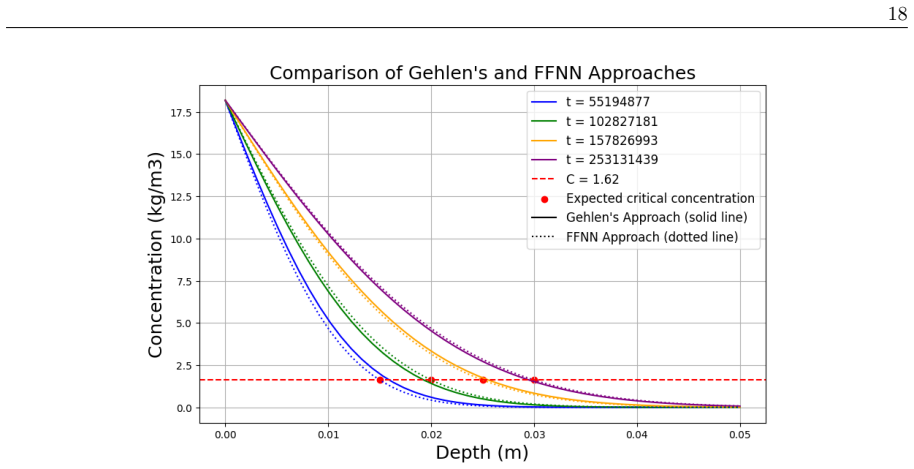
- The comparison shows that the physics-based model needs less data than the flexible neural network to generalize, and the two approaches could be combined to exploit both interpretability and flexibility.
Reading between the lines
- The 24-day lag and the 0.6 M% critical concentration are the main assumptions that convert resistance jumps into calibration pairs; replacing them with direct electrochemical depassivation measurements would make the method transferable to other structures without re-estimating these offsets.
- Because the neural network overfits with only four data points, adding more wire sensors at intermediate depths would allow a meaningful test of whether the data-driven approach catches up to the physics-based model as data grow.
- The model assumes one-dimensional, homogeneous diffusion; extending the calibration to cracked or layered concrete with a numerical solver would check whether the fitted parameters remain physically stable.
- A direct cross-validation on a second exposure cycle would test whether the calibrated diffusion coefficients predict the timing of new sensor breaks before they occur.
Editorial analysis
A structured set of objections, weighed in public.
Referee Report
Summary. The paper calibrates two models for chloride ingress into concrete using wire-sensor breakage times from the 'Concerto' test bridge: a physics-based Gehlen diffusion model with three parameters (a, Dt, be) estimated by Bayesian optimization, and a feed-forward neural network that maps time and temperature to an effective diffusion coefficient. The authors claim that progressive calibration with additional wire-sensor data yields increasingly accurate predictions of chloride penetration depth and that the calibrated diffusion coefficients agree with independent drilling-dust measurements. The paper also includes a Sobol sensitivity analysis, an optimizer sanity check, and a comparison against a rapid chloride migration (RCM) test.
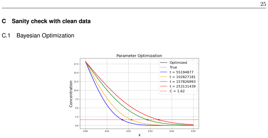
Significance. If the progressive-calibration claim were established, the work would be practically valuable for non-destructive corrosion monitoring of concrete infrastructure. The manuscript has genuine strengths: it uses multi-year real sensor data from a near-real-scale bridge, presents a transparent physics-based model, checks the Bayesian optimizer on synthetic data (Appendix C.1), and honestly acknowledges that the neural network is overfitted with four training points (Section 5.2). The commitment to publish data and code on Zenodo is also a positive feature. However, the central evidence for 'increasingly accurate predictions' is currently in-sample calibration, and the only independent comparison is sparse and not quantitatively evaluated. These load-bearing issues prevent the paper from supporting its main claim in its present form.
major comments (4)
- [Section 5.1, Eq. (10), Table 4, Figures 6-7] The demonstration of 'increasingly accurate predictions' is an in-sample calibration result, not a prediction on held-out data. In Table 4, the listed x_calc values equal the x_exp values by construction, because the optimization objective in Eq. (10) is the mean squared error over those exact depth-time pairs. Figures 6 and 7 plot the fitted model against the same points used for fitting. This does not support generalization to new wire depths or later exposure times. To substantiate the progressive-calibration claim, the authors should perform a genuine out-of-sample evaluation, such as leave-one-out calibration over the four points, or predict the deepest wire (0.03 m) using only the first three calibration points, and report quantitative predictive errors.
- [Section 5.4, Figure 13] The only non-circular validation is the comparison with drilling-dust-derived effective diffusion coefficients, but the text merely asserts 'good agreement' without a numerical tolerance or uncertainty band. Using the four-point calibrated parameters from Table 4 (a = 0.16, Dt = 1.29e-12 m2/s, be = 1010.7 K) in Eq. (4) gives DEff,C values on the order of 0.9e-12 and 0.6e-12 m2/s at t = 509 and 6692 days, respectively, whereas the chloride-profile regressions in Section 5.4 report 0.48e-12 and 0.12e-12 m2/s. The later value is therefore overestimated by roughly a factor of five. The paper should either quantify the discrepancy, provide confidence intervals from the parameter uncertainties, or explicitly state whether the discrepancy is expected within the CCrit uncertainty range shown in Figure 8.
- [Section 5.1, Table 4] The calibrated parameters are strongly unstable across the progressive-calibration steps: a varies from 0.10 to 0.78 and Dt from 1.18e-12 to 8.69e-12 m2/s. With only four data points and three free parameters, this indicates weak identifiability. This instability undermines the physical interpretation of the calibrated Dt and weakens the reliability claim made in Section 5.1. The authors should report parameter uncertainties or posterior ranges (for example, using the GP surrogate in the Bayesian optimizer), and they could implement the dimensionality reduction they propose in Section 3.1 by fixing be, then check whether the remaining parameters and predictions are stable.
- [Section 3, Assumption 2] The conversion of each resistance jump into a calibration point is load-bearing: the paper assumes that corrosion started exactly 24 days before the observed wire break and that at that earlier time the chloride concentration at the wire depth equaled 0.6 M% (1.62 kg/m3). This assumption turns every resistance jump into a depth-time observation used in Eq. (10). No sensitivity analysis or validation of the 24-day offset is provided, and the offset is not treated as an uncertain quantity. The authors should justify the offset with a quantitative reference or include it as an additional calibration parameter (or at least perturb it over a plausible range and show the effect on the fitted parameters and on the Section 5.4 comparison).
minor comments (7)
- [Section 3, Eq. (6)] The cosine argument in Eq. (6) is ambiguous because of the commas in the large numbers and the missing parentheses: '2π · t + 2, 542, 453.44 / 32, 407, 303.30' could be read as (2πt + 2,542,453.44) / 32,407,303.30 or as 2πt + (2,542,453.44 / 32,407,303.30). Please rewrite with clear parentheses and without thousands separators inside the mathematical expression.
- [Appendix C.1, Table 6] The text states that the true value of Dt is '2e-11', but Table 6 lists the true value as '2 × 10⁻¹²'. These are inconsistent and should be reconciled.
- [Section 1.2, Section 3] The wire is described as having a 'cross section area' of 0.065 mm, but mm is a unit of length, not area. Please specify either a diameter of 0.065 mm or give the cross-sectional area in mm2 (e.g., π·(0.0325 mm)2).
- [General formatting] Several table titles contain the typo 'T able' instead of 'Table' (e.g., Tables 1-3), and the heading 'Calibration using one Data pair' in Table 4 should read 'one data point'.
- [Section 5.2, Algorithm 2] The neural network training details are incomplete: the number of epochs, learning rate, and final loss value are not reported. Since the paper acknowledges overfitting, these details would help the reader judge the convergence claim.
- [Section 4] The description of fitting DEff,C from the chloride profiles says 'adjusting the calculated chloride concentration CS,Δx to the assumed chloride profile', which is unclear; it should clarify which parameters are adjusted in the nonlinear regression and how the uppermost layers are excluded.
- [References] Reference [11] is cited as 'DIN EN 12390-11:2015-11' but the standard number is 'DIN EN 12390-11'; also reference [6] is listed as a BAW data sheet without a full title or year, making it difficult to locate.
Circularity Check
The central 'increasingly accurate predictions' claim is demonstrated on the calibration set: Table 4 and Figures 6-7 compare fitted depths to the same measured depths that Eq. (10) minimizes over, so the progressive-calibration evidence is in-sample fit, not held-out prediction; the drilling-dust comparison is external but not quantified enough to rescue the claim.
-
fitted input called prediction
[Section 3.1, Eq. (10); Section 5.1, Table 4 and Figures 6-7]
"The aim of this optimization problem is to find the optimal parameters {a, be, Dt}∗ such that the the mean squared error (MSE) between the depths x according to 9 and the depths ˆxi of the measurement points listed in Table 2 is minimized. ... As seen in Figure 6, the calibration results show that the predicted depth aligns increasingly well with the observed data as more calibration points are added."
Equation (10) defines the fitted parameters as the minimizers of the discrepancy between computed and measured depths at exactly the four Table 2 points. Table 4 then reports x_calc equal to x_exp for those same points (0.015/0.015, 0.02/0.02, 0.025/0.025, 0.03/0.03), and Figures 6-7 plot the calibrated curve through those same measured points. Therefore the 'increasingly accurate predictions' shown are the in-sample residuals of the fitting objective, not out-of-sample predictions at new wire depths or times; the improvement is not evidence of generalization. The central progressive-calibration claim thus reduces to the fitting construction.
full rationale
The paper contains a genuine external element: the drilling-dust chloride profiles and RCM test in Section 5.4 are independent of the wire-sensor calibration, and the Gehlen model, the 24-day corrosion-start assumption, and the critical-chloride ranges are taken from external sources [1,5], not from the present authors' own prior work. No load-bearing self-citation chain is present. However, the main claim that progressive calibration with Bayesian optimization leads to increasingly accurate predictions is supported by Table 4 and Figures 6-7, which compare the fitted model to the same four points that Eq. (10) minimizes over. Table 4 lists x_calc = x_exp at each calibration stage by construction, and Figure 7, despite the word 'validation', is a calibration plot through those points. Thus the load-bearing demonstration of the central claim is in-sample fit. The only out-of-sample content is the extrapolated prediction curve in Figure 8 and the qualitative comparison with two drilling-dust diffusion coefficients in Section 5.4, but the latter is not quantified against the calibrated model's predictions with uncertainty bands. The score is 6 because one or more 'predictions' reduce by construction to the calibration objective, while the presence of independent external data prevents full circularity.
Assumptions & free parameters
free parameters (5)
- a (aging exponent in Gehlen model) =
≈0.16 (four-data-point calibration); ranges from ≈0.1 to ≈0.78 across calibrations
- Dt (transfer factor times migration coefficient, kt * DRCM,0) =
≈1.29e-12 m2/s (four-point calibration); ranges from ≈1.18e-12 to ≈8.69e-12
- be (temperature regression coefficient) =
≈1010.70 K (four-point calibration); ranges from ≈1000 to ≈2054
- Temperature model coefficients (offset, amplitude, phase, period) =
Offset=284.39 K, amplitude=11.10 K, phase=2542453.44 s, period=32407303.30 s in Eq. 6
- Neural network weights and biases (all θ) =
not reported, architecture 2-10-10-1 with ReLU, log-scaled output
assumptions (7)
- domain assumption Fick's second law with a time-dependent effective diffusion coefficient describes chloride ingress in concrete (Eq. 2 and Eq. 3).
- domain assumption The analytical error-function solution of Gehlen (Eq. 3) is valid for this concrete and exposure.
- ad hoc to paper A wire break indicates the wire fully corroded, and corrosion initiation occurred exactly 24 days before the break, at which time the chloride content at the wire depth equaled 0.6 M% (1.62 kg/m3).
- domain assumption The chloride surface concentration CS,Δx is 18.19 kg/m3 for the sensor data, derived from a 3 wt% NaCl solution.
- ad hoc to paper The internal concrete temperature follows the cosine regression in Eq. 6 with fixed coefficients.
- domain assumption For the dust sample regression, Fick's law with constant D applies, and the uppermost 5 mm (2007) and 20 mm (2024) are excluded as non-Fickian zones.
- domain assumption The critical chloride content CCrit is uncertain within 0.54 to 5.4 kg/m3 (0.2 to 2 M%), and all values in that range are treated as equally plausible.
Cite this review
Pith. "Pith review of Model-based reinforcement corrosion prediction: Continuous calibration with Bayesian optimization and corrosion wire sensor data." pith.science (2026). https://pith.science/paper/PWWCIAVZ
@misc{pith2026241116447,
  author       = {Pith},
  title        = {Pith review of: Model-based reinforcement corrosion prediction: Continuous calibration with Bayesian optimization and corrosion wire sensor data},
  year         = {2026},
  howpublished = {\url{https://pith.science/paper/PWWCIAVZ}},
  note         = {Machine review of arXiv:2411.16447}
}
read the original abstract
Chloride-induced corrosion significantly contributes to the degradation of reinforced concrete structures, making accurate predictions of chloride migration and its effects on material durability critical. This paper explores two modeling approaches to estimate the effective diffusion coefficient for chloride transport. The first approach follows Gehlen's interpretable diffusion model, which is based on established physical principles and incorporates time and temperature dependencies in predicting chloride migration. The second approach is a neural network-based method, where the neural network approximates the effective diffusion coefficient. In a subsequent step, the calibrated models are used to predict the penetration depth of the critical chloride content, taking into account the uncertainty in the critical chloride content. The models are calibrated using experimental data measured by a wire sensor installed in a concrete test bridge. The calibration results are compared to effective diffusion coefficients derived from drilling dust samples. A comparison of both approaches reveals the advantages of the physics-based model in terms of transparency and interpretability, while the neural network model demonstrates flexibility and adaptability in data-driven predictions. This study emphasizes the importance of combining traditional and machine learning-based methods to improve the accuracy of chloride migration predictions in reinforced concrete.
Figures


Figures from the paper (14 more)





Reference graph
Works this paper leans on
-
[1]
C. Gehlen, Probabilistische Lebensdauerbemessung von Stahlbetonbauwerken – Zu- verl¨ assigkeitsbetrachtungen zur wirksamen Vermeidung von Bewehrungskorrosion. DIN Media GmbH, 06 2000
work page 2000
-
[2]
Holst, Korrosionsmonitoring und Bruchortung vorgespannter Zugglieder in Bauwerken
A. Holst, Korrosionsmonitoring und Bruchortung vorgespannter Zugglieder in Bauwerken. PhD thesis, Institut f¨ ur Baustoffe, Massivbau und Brandschutz (IBMB), 2007
work page 2007
-
[3]
Monitoring von Betonbauwerken: Sensoren, Methoden, Erfahrungen,
Harald Budelmann, “Monitoring von Betonbauwerken: Sensoren, Methoden, Erfahrungen,” in Sicherheitsgewinn durch Monitoring?, Darmstadt: Freunde des Inst. f¨ ur Massivbau der TU, 2006
work page 2006
-
[4]
Korrosionsmonitoring von stahlbetonbauwerken mit einem funkbasierten drahtsensor,
I. Dressler, H.-J. Wichmann, and H. Budelmann, “Korrosionsmonitoring von stahlbetonbauwerken mit einem funkbasierten drahtsensor,” Bautechnik, vol. 92, no. 10, pp. 683–687, 2015
work page 2015
-
[5]
Korrosionsmonitoring von stahlbetonbauwerken als element des lebensdauermanagements,
A. Holst, H. Budelmann, and H.-J. Wichmann, “Korrosionsmonitoring von stahlbetonbauwerken als element des lebensdauermanagements,” Beton- und Stahlbetonbau, vol. 105, no. 12, pp. 536–549, 2010
work page 2010
-
[6]
BA W - Merkblatt: Dauerhaftigkeitsbemessung bei Carbon- atisierung und Chlorideinwirkung (MDCC)
Bundesanstalt f¨ ur Wasserbau - BA W, “BA W - Merkblatt: Dauerhaftigkeitsbemessung bei Carbon- atisierung und Chlorideinwirkung (MDCC).”
-
[7]
Chloride transport in concrete: theory and application,
R. F. M. Bakker, “Chloride transport in concrete: theory and application,” HERON, vol. 39, no. 1, pp. 45–83, 1994
work page 1994
-
[8]
Lausanne, Switzerland: CEB Bulletin No
Comit´ e Euro-International du B´ eton (CEB) Task Group V,Durability of Concrete Structures: State- of-the-Art Report. Lausanne, Switzerland: CEB Bulletin No. 238, 1997
work page 1997
Show all 20 references
-
[9]
Bayesian Optimization: Open source constrained global optimization tool for Python,
F. Nogueira, “Bayesian Optimization: Open source constrained global optimization tool for Python,” 2014–
2014
-
[10]
Goodfellow, Y
I. Goodfellow, Y. Bengio, and A. Courville, Deep Learning. online: MIT Press, 2016. https: //www.deeplearningbook.org
2016
-
[11]
DIN EN 12390-11:2015-11, Pr¨ ufung von Festbeton - Teil 11: Bestimmung des Chloridwiderstandes von Beton - Einseitig gerichtete Diffusion; Deutsche Fassung EN 12390-11:2015
“DIN EN 12390-11:2015-11, Pr¨ ufung von Festbeton - Teil 11: Bestimmung des Chloridwiderstandes von Beton - Einseitig gerichtete Diffusion; Deutsche Fassung EN 12390-11:2015.”
2015
-
[12]
Monte carlo and quasi-monte carlo sampling
S. U. Hai Wang Group, “Monte carlo and quasi-monte carlo sampling.” https://web.stanford. edu/group/haiwanglab/FFCM2/docs/ResponseSurface/MonteCarlo/, 2024. Accessed: 2024-11- 21. 21 A Calculations for CS,∆X The concentration of NaCl in the solution was determined based on a 3...
2024
-
[13]
Define the Problem : Specify the input parameters (i.e., be, Dt, and a) and their respective distribution (refer Subsection B.1). 23
-
[14]
The Sobol sampling algorithm ensures that the points are distributed uniformly, covering the range for each input parameter effectively
Generate Sobol Samples : • Sobol samples are quasi-random, low-discrepancy sequences that ensure good coverage of the input space with fewer samples than purely random sampling.[12] • For each input parameter, generate N samples and collect them in X. The Sobol sampling algori...
-
[15]
Evaluate the Model for Each Combination of x, t, and TIST: For each combination of x, t, and TIST, evaluate the model f (X) for all Sobol samples to obtain the output Y : Y = f (X). (20)
-
[16]
• Total-order Sobol indices S(j) T for be, Dt, and a, representing the total contribution of each parameter, including all interactions, for the j-th combination of data points
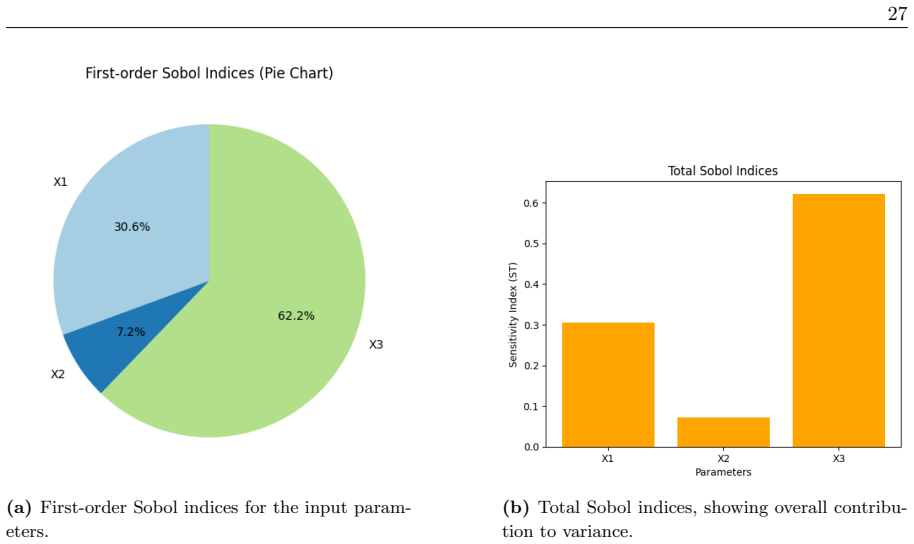
Perform Sobol Analysis : For each combination j, where j corresponds to a specific combination of depth x, time t, and temperature TIST as listed in Table 2, calculate: • First-order Sobol indices S(j) 1 for be, Dt, and a, representing the independent effect of each parameter ...
-
[17]
• Xi represents the i-th input parameter ( be, Dt, or a)
V alidate V ariance Decomposition: For each combination j, check if the sum of first-order Sobol indices S1 approximates the total variance V (Y ) by verifying: Variance Sum(j) = kX i=1 S(j) 1 (Xi) × V (Y (j)) ≈ V (Y (j)), (21) where: • j refers to a specific combination of x,...
-
[18]
• m is the total number of combinations of x, t, and TIST as defined in Table 2
Average Sobol Indices Across All Runs : Compute the average first-order S1 and total-order ST indices across all combinations of x, t, and TIST (indexed by j) for each input parameter ( be, Dt, and a)(indexed by i): Average S1(Xi) = 1 m mX j=1 S(j) 1 (Xi), Average ST (Xi) = 1 ...
-
[19]
Plot Results: Plot the averaged first-order Sobol indices S1 and total-order Sobol indices ST as bar charts
-
[20]
Return Results: Return a dictionary containing S1 and ST averaged over all runs. The Sobol sensitivity analysis revealed that the first-order as well as the total-order Sobol index for a was the highest, followed by Dt, with the least contribution by be, confirming its dominan...
Reviewed August 12, 2026 · model on record in the stance chip above.
Discussion (0). Continue with ORCID to comment.