REVIEW 4 major objections 6 minor 2 references
Statistical Emulations of Human Operational Motions in Industrial Environments
T0 review · 4 major / 6 minor · reviewed 2026-08-12 · deepseek-v4-flash
Pith's one-line read The paper claims that a flatten-then-Gaussian pipeline can generate statistically faithful industrial motion sequences from about 60 training sequences per task class.
desk verdict Solid flatten-and-Gaussian methods contribution with a genuinely new IS-TVF representation, but the realism claim outruns the evidence: the model never samples time warping, the real-data tests mostly reject, and the synthetic benchmark is circular. read the letter →
The pith
A machine-rendered reading of the paper's core claim, the machinery that carries it, and where it could break.
The reading
What carries the argument
The load-bearing chain is: represent each motion as $\alpha:[0,1]\to\mathcal{Y}$, where $\mathcal{Y}$ is a product of unit spheres, one per body landmark, after removing location and scale; align all sequences to a reference by S-TSRVF time warping; flatten either by IS-TVF (integrated single-hop transported velocity field, parallel-transport each shooting vector to the reference tangent space and integrate) or SIEM (single inverse exponential map, map each posture directly to the reference tangent space); reduce dimension by sequential PCA, meaning spatial PCA followed by functional PCA; and impose a multivariate Gaussian on the resulting $d_1\times d_2$ coefficients. Because every map in the chain is invertible, sampling coefficients and applying the inverse maps yields a full new motion sequence.
What would settle it
Estimate the optimal time-warping functions $\gamma$ from the training sequences; if their distribution has substantial spread and the emulator's generated sequences cannot reproduce that spread, for instance a two-sample test on $\gamma$ rejects, the claim that the emulator reproduces real operational motions fails on execution-rate variability.
Extended reading notes
Core claim
The central claim is that, once human motion is treated as a curve on the shape manifold of body postures, temporal alignment plus a bijective flattening into a tangent space reduces the emulation problem to sampling a Gaussian distribution over a small set of PCA coefficients. The paper introduces IS-TVF and SIEM as two flattening maps, combines them with sequential spatial-plus-functional PCA, and shows that the resulting emulator produces smooth, class-appropriate skeleton sequences whose distribution matches the training data better than an intrinsic pointwise Gaussian model or a vector autoregressive model. The best performing configuration is SIEM/SequentialPCA/MVG.
Load-bearing premise
The pipeline assumes that time-warping alignment fully removes execution-rate differences, so the generative model never has to produce speed variation; if realistic emulation must include different work speeds, this assumption breaks.
Editorial extensions
If this is right
- A digital twin of a manual workstation could draw unlimited synthetic motion sequences for a given task class from as few as 60 recorded sequences, enabling operations planning and worker-effort optimization without more data collection.
- Generated sequences inherit the smoothness and posture statistics of the training class, so downstream planners can use them as representative human-induced process variation.
- Because the representation is bijective, the same pipeline can be reused as a generative model for human body shapes generally, not only for the five manufacturing classes tested.
- The comparisons rank the pointwise intrinsic model and the vector autoregressive model below the flatten-plus-Gaussian schemes, indicating that temporal correlation is better captured by the PCA-coefficient Gaussian than by pointwise independence or a fixed-lag autoregression.
Reading between the lines
- The paper never models or samples the time-warping functions; it assumes alignment removes phase. An obvious extension is to estimate the distribution of $\gamma$ from training data and sample it alongside the shape coefficients, which would let the emulator reproduce execution-rate variability, a challenge the paper itself lists.
- The multivariate Gaussian on PCA coefficients is unimodal; for motion classes with several distinct sub-actions, a mixture or latent-variable model on the coefficients would likely improve fidelity, and the quantization evaluation hints at this by showing cluster transitions.
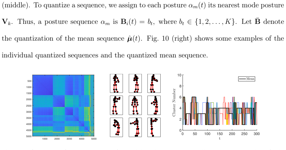
- The quantization metric could be turned into a pre-deployment acceptance test: an emulated sequence is usable if its posture-cluster sequence is statistically indistinguishable from real task-cluster sequences.
Editorial analysis
A structured set of objections, weighed in public.
Referee Report
Summary. The paper develops a pipeline for simulating human operational motion sequences in industrial settings. Human postures are represented as elements of a product-of-spheres shape space, and motion sequences as paths in that space. The pipeline temporally aligns sequences using S-TSRVF-based warping, flattens the aligned shape sequences into Euclidean representations (the proposed IS-TVF and the existing SIEM), reduces dimension with sequential spatial/functional PCA, and then fits statistical models (multivariate Gaussian, independent Gaussian, VAR, or a point-wise intrinsic model) to the reduced coefficients. New sequences are generated by sampling from these models and inverting the flattening/PCA maps. The method is evaluated on a five-class manufacturing motion dataset using visualization, MDS plots, DISCO two-sample tests, log-likelihood comparisons, a two-level simulation study, and a posture-quantization metric.
Significance. The paper's mathematical core is a strength: the flattening maps are defined explicitly, the reconstruction pipeline is invertible, and the numerical experiments show that single-hop flattenings (S-TVF/IS-TVF and SIEM) reconstruct sequences with errors around 10^-7, whereas multi-hop transport accumulates visible distortion. The systematic comparison of representation, dimension-reduction, and stochastic-model choices is useful for practitioners building digital twins of manual operations. The proposed IS-TVF is a reasonable new representation. However, the central claim that the resulting emulator produces sequences that are statistically and visually realistic is not established by the evidence as presented: the real-data two-sample tests mostly reject distributional equality, the level-two 'benchmark' is generated by the same family of models being evaluated, and the generative model never samples the time-warping function that the abstract itself identifies as a key source of variability. These issues affect the paper's main claim rather than the internal consistency of the derivations.
major comments (4)
- [§5.2, Table 2] The DISCO two-sample tests on real motion-class-one sub-sequences mostly reject the null hypothesis that simulated and observed sequences have the same distribution: p-values for IS-TVF/SequentialPCA/MVG are 0.0211, 0.0109, and 0.0012, and for SIEM/SequentialPCA/MVG they are 0.0544, 0.0190, and 0.0022, with the VAR model at exactly 0. The text acknowledges that 'the p-values were still small.' Since the conclusion in §6 states that these models 'simulate realistic motion sequences' and that SIEM 'performs the best,' the manuscript should either substantially temper the realism claim to a relative-model-comparison statement or provide an explicit argument for why rejection of distributional equality is compatible with the intended downstream use. As written, the paper's own headline evaluation does not support the headline claim.
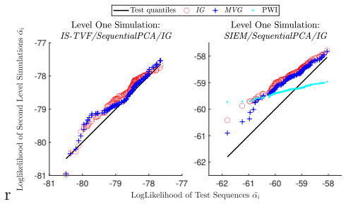
- [§5.3, Fig. 14, Table 3] The two-level simulation study is circular with respect to the realism claim. The 'benchmark' training and test sets in level two are not real human motions; they are sequences generated by IS-TVF/SequentialPCA/IG or SIEM/SequentialPCA/IG in level one. The emulators evaluated in level two are then fitted to and compared against these synthetic data, and the high p-values in Table 3 show only that the same parametric family can resample its own outputs. This validates internal consistency and computational reproducibility, not closeness to human operational motion. The paper should clearly separate this internal-consistency check from validation against real data, or replace the level-two benchmark with independently collected or held-out real data.
- [§3.2, §4.3] The generative model omits the phase component that the paper itself lists as a core challenge. Section 3.2 computes an optimal time warping for each training sequence and then states, 'From here onwards, we will assume that all the sequences are temporally aligned.' The generative stage in §4.3 samples PCA coefficients and reconstructs aligned shape sequences; it never estimates or samples a distribution over time-warping functions. The abstract lists 'variability in execution rates across observations' as one of the key challenges, and Fig. 2 motivates exactly this phenomenon. Because the DISCO tests in Table 2 compare sequences in the aligned representation, they cannot detect the missing phase variability. If the intended target is explicitly time-normalized shape sequences, the paper must restate its scope; otherwise, the emulator is structurally incapable of reproducing execution-rate variation and the realism claim is overbroad.
- [§5.4, Table 4] The quantization-based metric is interpreted in a way that does not follow from its definition. The quantity E(m) in §4.4 measures disagreement between a quantized sequence and the quantized mean sequence, so smaller values mean 'closer to the mean,' not 'closer to the original distribution.' In Table 4, the PWI model has the smallest mean variability in four of five motion classes (e.g., 0.2110 versus the original 0.2911 in Motion 1), which is consistent with the paper's own observation that PWI generates sequences concentrated around the mean. A smaller E value is therefore not evidence of better emulation; it can indicate overconcentration. The table should be reinterpreted or replaced with a statistic that measures distributional discrepancy, such as a two-sample test on quantized sequences.
minor comments (6)
- [§4.1] The heading contains a typo: 'Mathmetical Representation' should read 'Mathematical Representation.'
- [Definition 4.1] The codomain of Gα is written as T_{α(0)}(Y), but the preceding paragraph states that S-TVF values Fα lie in T_{YR}(Y), and the reconstruction procedure uses that same tangent space. The codomain should be T_{YR}(Y) for consistency.
- [Eq. (4)] The displayed Gaussian log-likelihood is missing the minus sign in the quadratic term and the normalizing constants. As written, 'exp(1/2 vec(A*)⊤Σ^{-1}vec(A*))' grows with the Mahalanobis distance instead of decaying; the formula should be -(d/2)log(2π) - (1/2)log det(Σ) - (1/2)vec(A*)⊤Σ^{-1}vec(A*).
- [Fig. 12] The four MDS plots are computed independently for each panel, so the degree of overlap between red and blue points is not comparable across panels; a single joint embedding would provide stronger visual evidence for the claim that some models cover the training distribution better than others.
- [Tables 1 and 2] There are spacing artifacts in the table headings ('T able 1' and 'I S-TVF/Spa-tialPCA/V AR') that should be corrected.
- [§5.4] The sentence 'There are 90,300 individual postures in total from all the five motion classes' is unclear until one computes 60 sequences × 301 time points × 5 classes; the wording should be explicit about how this number is obtained.
Circularity Check
Level-two 'benchmark' is generated by the same IS-TVF/SIEM-PCA-Gaussian family being evaluated, so the high p-values in Table 3 validate self-consistency, not realism.
-
fitted input called prediction
[Section 5.3 (Further Simulation and Evaluation), Fig. 14 pipeline and Table 3]
"we use 60 observed sequences in motion class one to fit a model and then sample this fitted model to generate 1000 new sequences {˜αi}. We randomly divide them into a training set (800 sequences) and a test set (200 sequences). Here we focus only on IS-TVF/SequentialPCA/IG and SIEM/SequentialPCA/IG models. ... Each statistical emulator is fitted using the training set of the benchmark dataset, and the fitted emulator is used to simulate 200 sequences {ˆαi}, which we refer to as the level-two simulation data."
The 'benchmark test set' in this two-level simulation is not independent real data; it is sampled from a level-one model that is itself one of the same representation/PCA/Gaussian families (IS-TVF/SequentialPCA/IG or SIEM/SequentialPCA/IG) that the level-two emulators instantiate. The level-two emulators are fitted on a synthetic training set generated from that same family and then validated against a synthetic test set drawn from the same family. High p-values in Table 3 therefore show that a model from the family can reproduce another draw from the same family, which is forced by construction. This is a self-consistency check of the estimation procedure, not evidence that the emulator matches real human operational motion.
full rationale
The core derivation—S-TSRVF temporal alignment, IS-TVF/SIEM flattening, sequential PCA dimension reduction, Gaussian coefficient modeling, and reconstruction through bijective maps—is not circular: each component is defined and estimated independently, and reconstruction fidelity is checked against the original training data with explicit error measures (Fig. 5, Table 1). The simplification in Section 3.2, 'we will assume that all the sequences are temporally aligned,' is a stated scope limitation rather than a circular step: the generative model never samples time-warping functions, which is a completeness gap for execution-rate variability, not a definitional equivalence. No load-bearing uniqueness theorem is imported through self-citation, and the TSRVF alignment machinery is standard external methodology with independent support. The genuine circularity is confined to the evaluation: Section 5.3 constructs the level-one benchmark by sampling from a fitted IS-TVF/SequentialPCA/IG or SIEM/SequentialPCA/IG model, then fits level-two emulators from the same model family and reports high p-values against the synthetic test set. Those p-values are forced by construction because the test distribution is itself a draw from the model class under test; they establish internal consistency, not fidelity to real human motion. This partial circularity in the validation of the realism claim prevents a lower score, while the central derivation remains self-contained.
Assumptions & free parameters
free parameters (6)
- PCA spatial dimension d1 =
10 (subsequences: 8, 10, 12; level-two: 4)
- PCA temporal dimension d2 =
30 (subsequences: 4, 5, 10; level-two: 4)
- Number of posture clusters K =
9
- VAR order p =
4
- Downsampled sequence length T =
301 (from 1000)
- Reference posture Y_R =
unspecified
assumptions (7)
- standard math Riemannian geometry of the product-of-spheres shape space Y = (S^2)^(n-1): exponential/log maps and parallel transport along geodesics are valid and invertible enough for reconstruction.
- domain assumption The S-TSRVF time-warping alignment finds an optimal gamma and fully synchronizes sequences with no residual phase variability relevant to downstream modeling.
- domain assumption A multivariate Gaussian on PCA coefficients adequately represents the population of motion sequences.
- domain assumption Temporal alignment and flattening can be performed separately per class, and the reference/tangent space distortions are negligible.
- standard math The DISCO two-sample test and permutation procedure give valid p-values for the sequence distances used.
- domain assumption The available 60 sequences per class are sufficient to estimate the PCA covariance and Gaussian parameters.
- domain assumption Human posture can be represented by normalized landmark directions, discarding body size, proportions and location.
Cite this review
Pith. "Pith review of Statistical Emulations of Human Operational Motions in Industrial Environments." pith.science (2026). https://pith.science/paper/CVL5HEJI
@misc{pith2026241116929,
  author       = {Pith},
  title        = {Pith review of: Statistical Emulations of Human Operational Motions in Industrial Environments},
  year         = {2026},
  howpublished = {\url{https://pith.science/paper/CVL5HEJI}},
  note         = {Machine review of arXiv:2411.16929}
}
read the original abstract
This paper tackles the challenging problem of developing emulators for human operational motions in industrial workplaces. We represent human motion as time-indexed sequences of body shapes and formulate a statistical generative model for these shape sequences. The sequences are modeled as continuous-time stochastic processes on a Riemannian shape manifold. Key challenges include the manifold's nonlinearity, variability in motion execution rates, the infinite-dimensional nature of the processes, and population-level variability across action classes. Deep learning methods are ineffective due to the small training samples typically available in this domain. To address these issues, we integrate a number of tools: temporal alignment via time warping, Riemannian geometry for handling nonlinearities, and shape- and functional-PCA for dimensionality reduction. A Gaussian model is then imposed on the reduced Euclidean spaces to emulate random motion sequences, which are then evaluated in representative industrial scenarios. We utilize a number of metrics to validate randomly generated shape sequences.
Figures


Figures from the paper (14 more)






Reference graph
Works this paper leans on
-
[1]
17 shows the detailed simulation process for the IS-TVF/SequentialPCA/MVG model
IS-TVF/SequentialPCA/MVG: Fig. 17 shows the detailed simulation process for the IS-TVF/SequentialPCA/MVG model. While the simulated spatial PCA coefficient trajec- tories H∗ αm (the first panel) and IS-TVF functions G∗ αm (the second panel) are similar to the original functions, the simulated S-TVF functionsG∗ αm (the third panel) are much smoother than t...
-
[2]
18 shows the simula- tion process of SIEM/SequentialPCA/MVG model
SIEM/SequentialPCA/MVG: Similar to the previous case, Fig. 18 shows the simula- tion process of SIEM/SequentialPCA/MVG model. The top panel shows the simulated spatial PCA coefficient trajectories H∗ αm, and the middle shows the SIEM functions W∗ αm. In contrast to the IS-TVF approach, the simulated SIEM functions W∗ αm have a similar smoothness as the or...
Reviewed August 12, 2026 · model on record in the stance chip above.
Discussion (0). Continue with ORCID to comment.