REVIEW 2 major objections 5 minor 38 references
Quantile Graph Discovery through QuACC: Quantile Association via Conditional Concordance
T0 review · 2 major / 5 minor · reviewed 2026-08-12 · deepseek-v4-flash
Pith's one-line read The paper introduces QuACC, a statistic measuring whether two variables are jointly above (or below) their conditional quantiles, proves asymptotic normality for plug-in estimators, and uses it as a conditional-association test inside a…
desk verdict QuACC is a sensible idea for tail-specific association graphs, but the key variance term in the test statistic is wrong, and the graph semantics are looser than claimed. read the letter →
The pith
A machine-rendered reading of the paper's core claim, the machinery that carries it, and where it could break.
The reading
What carries the argument
The central object is the QuACC concordance probability, defined as the joint probability that two variables fall on the same side of their conditional quantile functions at level $\tau$. The machinery around it is a cross-fitted plug-in estimator: fit quantile regressions for $Y$ and $X$ on training folds, evaluate indicator concordance on a held-out fold, then pool folds. The proof machinery is a decomposition of estimation error into a testing-set concordance term with variance $V(\tau)$ and a quantile-estimation term with covariance $V_{XY}(\tau)$ weighted by density factors $\kappa_Y,\kappa_X$; Theorem 1 says the sum is asymptotically normal. This normality is what converts QuACC into a $z$-test and lets the PC algorithm use it as a conditional-independence oracle at each quantile level.
What would settle it
Take independent standard normal variables with no conditioning set and $\tau=0.5$: the paper's Lemma 2 gives $V(\tau)=\tau^2(1-\tau)^2=0.0625$, while direct computation gives $\mathrm{Var}(I(Y<0)I(X<0))=(0.25)(0.75)=0.1875$, showing the variance formula in Theorem 1 does not match the variance of the observed concordance statistic.
Extended reading notes
Core claim
The central claim is that for fixed $\tau$, the QuACC statistic $\rho_\tau(Y,X|Z)=P(Y>Q_Y(\tau|Z),\,X>Q_X(\tau|Z))$ for $\tau\ge 0.5$ (and the analogous lower-tail probability for $\tau<0.5$) is a meaningful, testable quantile-specific conditional association. Under conditions C1-C4, the cross-fitted plug-in estimator $\hat{\rho}^k_\tau$ satisfies $(b_n)^{1/2}(\hat{\rho}^k_\tau-\rho_{\tau 0})\to N(0,\Sigma_\tau)$ with $\Sigma_\tau=\kappa_Y\sigma^2_{Q_Y}\kappa_Y+\kappa_X\sigma^2_{Q_X}\kappa_X+2\kappa_Y\kappa_X V_{XY}(\tau)+V(\tau)$, where $\kappa_Y,\kappa_X$ encode derivatives of the concordance probability with respect to the quantile functions, $V_{XY}(\tau)$ captures the joint estimation error of the two quantile regressions, and $V(\tau)$ is the variance of the concordance indicators at the true quantiles. For linear quantile regression a root-$n$ version is given, yielding a standard-normal test statistic for $H_0:\rho_\tau=(1-\tau)^2$ (upper) or $\tau^2$ (lower). The intended use is not just pairwise testing: feeding this test statistic into the PC algorithm produces a quantile-specific graphical model whose missing edges denote conditional independence at that quantile.
Load-bearing premise
The whole inference rests on the claim that subtracting each variable's exceedance probability before multiplying does not change the variance of the joint-exceedance indicator; the variance formulas in Theorem 1 are valid only if this algebraic identity holds.
Editorial extensions
If this is right
- If the central claim is right, researchers can test whether two variables move to their extremes together given a covariate set, using a standard normal statistic at any $\tau$ and no assumed copula family.
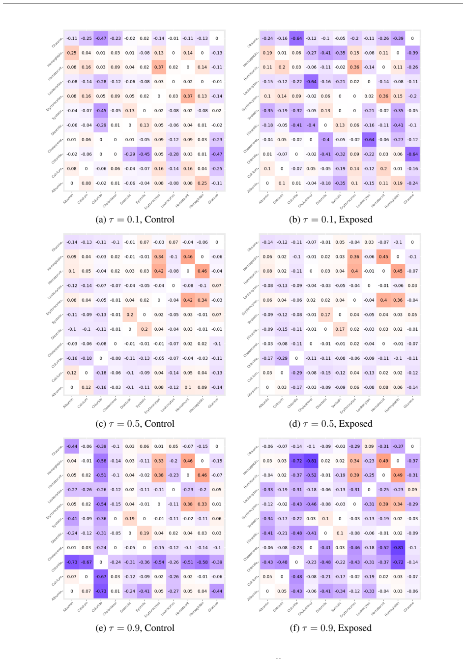
- Running the test inside the PC algorithm yields one undirected skeleton per quantile level; edges present at $\tau=0.9$ but absent at $\tau=0.5$ would mark tail-only conditional associations.
- The same plug-in logic extends the graph framework to nonlinear quantile regressions such as quantile forests, at the cost of a slower $(n/s)^{1/2}$ convergence rate.
- Applied to biobank biomarker panels, the method can produce quantile-specific graphs that differ at lower and upper tails, which is where dysregulation is often visible.
- Correct estimation of the conditional quantile functions is a precondition for the null benchmark $(1-\tau)^2$ or $\tau^2$ to be valid, so the test is only as reliable as the fitted quantile models.
Reading between the lines
- The paper tests one pair of quantiles at a time; a natural extension would be a joint test over a grid of $\tau$ values, which would detect dependence appearing at any tail without the multiple-testing burden of separate tests.
- The concordance definition could be generalized to asymmetric quantile levels $\tau_Y\ne\tau_X$, allowing questions such as whether upper-tail movement in one variable tracks lower-tail movement in another; the variance decomposition would need a new $V(\tau)$ term.
- If the asymptotic result extends, QuACC could serve as a screening statistic before fitting full conditional copula models, since it targets precisely the corner probabilities that copulas aim to capture.
- The graph produced by the PC skeleton at one $\tau$ should be read as quantile-specific association structure, not as full causal structure; orienting edges and combining layers across $\tau$ would require additional assumptions the paper does not state.
Editorial analysis
A structured set of objections, weighed in public.
Referee Report
Summary. The paper introduces QuACC (Quantile Association via Conditional Concordance), a measure of quantile-specific conditional association defined as the probability that two variables jointly exceed (or fall below) their conditional quantile functions at level tau. The authors propose a cross-fitted plug-in estimator, claim asymptotic normality of the estimator (Theorem 1 and Corollary 1.1), and use this result to build Wald tests for the null hypothesis of independence, rho_tau = (1-tau)^2 or tau^2. These tests are then plugged into the PC algorithm to estimate undirected skeletons for what the authors call QuACC graphical models (QGMs). The method is evaluated in simulations and applied to All of Us biobank data for mitochondrial disorders.
Significance. If the asymptotic theory were correct, QuACC would provide a practically useful tool for detecting tail-specific conditional associations and for constructing quantile-level graphical models, complementing existing quantile graphical model approaches. The paper has several strengths: it uses cross-fitting to separate nuisance estimation from inference, it accommodates both linear and random-forest quantile regressions, it includes simulation studies across copula settings, and it demonstrates a real-data application. However, the central variance derivation in Lemma 2 is algebraically incorrect, and the resulting test statistic and graphical outputs are not valid. The paper's main contribution therefore rests on an unsupported claim.
major comments (2)
- [Appendix F, Lemma 2; Section 2.2, Theorem 1 and hypothesis test] The proof of Lemma 2 asserts that Var(I(Y<QY)I(X<QX)) = Var((I(Y<QY)-tau)(I(X<QX)-tau)). This identity is false: for independent Bernoulli(tau) indicators A and B, Var(AB) = tau^2(1-tau^2), whereas Var((A-tau)(B-tau)) = tau^2(1-tau)^2. At tau=0.5 the former is 0.1875 and the latter 0.0625, a factor of three. The subsequent algebra also sets (E[W1W2])^2 = tau^2(1-4tau+4tau^2), but E[W1W2] = p(Y<QY, X<QX) - tau^2, which is zero under independence, not tau^2(1-2tau)^2. Because V(tau) enters Theorem 1 and Corollary 1.1, the null variance used in the z-statistic (Section 2.2, Hypothesis test) is too small, leading to inflated Type I error. The simulation rejection rates in Section 3.1 and the QGM graphs in Section 4 therefore do not provide valid evidence of the method's performance.
- [Section 2.3, QuACC Graphical Models] The PC algorithm requires a test of conditional independence to decide edge removal. The paper instead tests H0: rho_tau = (1-tau)^2 (or tau^2), which is a single condition on the joint exceedance probability, not a statement of full conditional independence of Y and X given Z. The paper does not prove that accepting this null is equivalent to, or even implies, the conditional independence required for the PC algorithm's edge-removal step. Without such a formal connection, the output of the QGM procedure lacks a well-defined interpretation as a conditional independence graph, and the manuscript's central graphical-model claim is unsupported.
minor comments (5)
- [Section 2.1, equation for overall b-rho] The displayed formula for b-rho_tau after defining b-rho^k_tau appears malformed: "bρτ = PK k=1 bρk τqPK k=1 V ar(bρkτ )/nk" is missing an operator and is not a valid expression. Please rewrite it unambiguously.
- [Appendix C, last paragraph] The sentence "If they are perfectly discordant, ie. they ever jointly above or below their regression planes, then ρ∗τ is 1" should say "never jointly" and the value should be -1, consistent with the normalization formula.
- [Introduction, Section 1] The text states that a negative rho_tau indicates discordance and that the smallest possible rho_tau is 0, but the definition of rho_tau as a probability is always nonnegative. Please clarify that only the normalized version rho*_tau can take negative values, and correct the related discussion.
- [Theorem 1 proof, page 21] The variance term for In2 is written as "2κYκX nk VXY(τ)" in the proof but as "2κYκX VXY(τ)" in the theorem statement. The factor 1/nk (if intended) should be specified precisely, since it affects the asymptotic variance expression.
- [References and typos] There are several typographical errors: "V owels" in the references should be "Vowels"; "Ceber's optic atrophy" should be "Leber's optic atrophy"; and the notation "≶" in Lemma 2 is unclear without specifying lower versus upper tail cases.
Circularity Check
No significant circularity: QuACC's null values are derived from independence, not fitted; the variance-formula error is algebraic, not circular.
full rationale
The QuACC construction is self-contained: the statistic is defined directly as a joint exceedance concordance probability, and the null value (1-tau)^2 or tau^2 is obtained by multiplying Bernoulli exceedance probabilities under independence, not by fitting any parameter to data. The asymptotic distribution in Theorem 1 is built from a Taylor expansion of the concordance function plus a central limit theorem applied to test-fold indicators, with the quantile-regression nuisance components supplied by standard external results (Koenker and Hallock, Athey et al.). The paper does not invoke a prior uniqueness theorem, does not rely on a self-citation chain, and does not rename a fitted quantity as a prediction; the simulations use known copula parameters to assess power rather than to calibrate the method. The reader-identified flaw in Lemma 2, that Var(I(Y<QY)I(X<QX)) is not equal to Var((I(Y<QY)-tau)(I(X<QX)-tau)), is a genuine algebraic error affecting the Wald denominator and downstream Type I error, but it is a mathematical mistake rather than a circular reduction of the conclusion to the inputs. Similarly, the unproven semantic step from accepting the single-probability null rho_tau = tau^2 to PC edge removal concerns statistical validity, not circularity. No circular step can be exhibited by quoting the paper's equations as equivalent by construction, so the circularity score is 0.
Assumptions & free parameters
free parameters (3)
- number of cross-fitting folds K =
5
- bandwidth hn for density estimation =
Hall-Sheather O(n^{-1/3}) or Bofinger O(n^{-1/5})
- quantile level tau =
user-specified, e.g., 0.1, 0.5, 0.9
assumptions (4)
- domain assumption Conditions C1-C4 (bounded moments, continuous densities, consistent quantile estimators, differentiable joint CDF) hold.
- domain assumption The conditional quantile models QY(tau|Z) and QX(tau|Z) are correctly specified.
- ad hoc to paper In the PC algorithm, failing to reject H0: rho_tau=c is treated as evidence for conditional independence.
- domain assumption Faithfulness and the other standard PC assumptions hold for the quantile-concordance graph.
Cite this review
Pith. "Pith review of Quantile Graph Discovery through QuACC: Quantile Association via Conditional Concordance." pith.science (2026). https://pith.science/paper/PCP3XGFQ
@misc{pith2026241117033,
  author       = {Pith},
  title        = {Pith review of: Quantile Graph Discovery through QuACC: Quantile Association via Conditional Concordance},
  year         = {2026},
  howpublished = {\url{https://pith.science/paper/PCP3XGFQ}},
  note         = {Machine review of arXiv:2411.17033}
}
read the original abstract
Graphical structure learning is an effective way to assess and visualize cross-biomarker dependencies in biomedical settings. Standard approaches to estimating graphs rely on conditional independence tests that may not be sensitive to associations that manifest at the tails of joint distributions, i.e., they may miss connections among variables that exhibit associations mainly at lower or upper quantiles. In this work, we propose a novel measure of quantile-specific conditional association called QuACC: Quantile Association via Conditional Concordance. For a pair of variables and a conditioning set, QuACC quantifies agreement between the residuals from two quantile regression models, which may be linear or more complex, e.g., quantile forests. Using this measure as the basis for a test of null (quantile) association, we introduce a new class of quantile-specific graphical models. Through simulation we show our method is powerful for detecting dependencies under dependencies that manifest at the tails of distributions. We apply our method to biobank data from All of Us and identify quantile-specific patterns of conditional association in a multivariate setting.
Figures


Figures from the paper (11 more)




Reference graph
Works this paper leans on
-
[1]
The multiple quantile graphical model
Alnur Ali, J Zico Kolter, and Ryan J Tibshirani. The multiple quantile graphical model. Advances in Neural Information Processing Systems, 29, 2016
work page 2016
- [2]
-
[3]
Generalized random forests
Susan Athey, Julie Tibshirani, and Stefan Wager. Generalized random forests. The Annals of Statistics, 47 0 (2): 0 1148--1178, 2019
2019
-
[4]
Alexandre Belloni, Mingli Chen, and Victor Chernozhukov. Quantile graphical models: Prediction and conditional independence with applications to financial risk management. 2016
work page 2016
-
[5]
Optimal condensation of distributions and optimal spacing of order statistics
Eve Bofinger. Optimal condensation of distributions and optimal spacing of order statistics. Journal of the american statistical association, 70 0 (349): 0 151--154, 1975
work page 1975
-
[6]
Network analysis: an integrative approach to the structure of psychopathology
Denny Borsboom and Ang \'e lique OJ Cramer. Network analysis: an integrative approach to the structure of psychopathology. Annual review of clinical psychology, 9: 0 91--121, 2013
work page 2013
-
[7]
Quantile regression neural networks: Implementation in r and application to precipitation downscaling
Alex J Cannon. Quantile regression neural networks: Implementation in r and application to precipitation downscaling. Computers & geosciences, 37 0 (9): 0 1277--1284, 2011
2011
-
[8]
Nonparametric causal structure learning in high dimensions
Shubhadeep Chakraborty and Ali Shojaie. Nonparametric causal structure learning in high dimensions. Entropy, 24 0 (3): 0 351, 2022
work page 2022
Show all 38 references
-
[9]
Quantile association regression on bivariate survival data
Ling-Wan Chen, Yu Cheng, Ying Ding, and Ruosha Li. Quantile association regression on bivariate survival data. Canadian Journal of Statistics, 49 0 (3): 0 612--636, 2021
2021
-
[10]
Double/debiased machine learning for treatment and structural parameters, 2018
Victor Chernozhukov, Denis Chetverikov, Mert Demirer, Esther Duflo, Christian Hansen, Whitney Newey, and James Robins. Double/debiased machine learning for treatment and structural parameters, 2018
2018
-
[11]
Sparse graphical models for exploring gene expression data
Adrian Dobra, Chris Hans, Beatrix Jones, Joseph R Nevins, Guang Yao, and Mike West. Sparse graphical models for exploring gene expression data. Journal of Multivariate Analysis, 90 0 (1): 0 196--212, 2004
2004
-
[12]
Levels of pathogen virulence and host resistance both shape the antibody response to an emerging bacterial disease
Daisy E Gates, Molly Staley, Luc Tardy, Mathieu Giraudeau, Geoffrey E Hill, Kevin J McGraw, and Camille Bonneaud. Levels of pathogen virulence and host resistance both shape the antibody response to an emerging bacterial disease. Scientific reports, 11 0 (1): 0 8209, 2021
2021
-
[13]
Conditional copulas, association measures and their applications
Ir \`e ne Gijbels, No \"e l Veraverbeke, and Marel Omelka. Conditional copulas, association measures and their applications. Computational Statistics & Data Analysis, 55 0 (5): 0 1919--1932, 2011
1919
-
[14]
Quantile graphical models: a Bayesian approach
Nilabja Guha, Veera Baladandayuthapani, and Bani K Mallick. Quantile graphical models: a Bayesian approach. The Journal of Machine Learning Research, 21 0 (1): 0 3023--3069, 2020
2020
-
[15]
On the distribution of a studentized quantile
Peter Hall and Simon J Sheather. On the distribution of a studentized quantile. Journal of the Royal Statistical Society: Series B (Methodological), 50 0 (3): 0 381--391, 1988
1988
-
[16]
PC algorithm for nonparanormal graphical models
Naftali Harris and Mathias Drton. PC algorithm for nonparanormal graphical models. Journal of Machine Learning Research, 14 0 (11), 2013
2013
-
[17]
The elements of statistical learning: data mining, inference, and prediction, volume 2
Trevor Hastie, Robert Tibshirani, Jerome H Friedman, and Jerome H Friedman. The elements of statistical learning: data mining, inference, and prediction, volume 2. Springer, 2009
2009
-
[18]
On parameters of increasing dimensions
Xuming He and Qi-Man Shao. On parameters of increasing dimensions. Journal of multivariate analysis, 73 0 (1): 0 120--135, 2000
2000
-
[19]
Current research trends in early life stress and depression: Review of human studies on sensitive periods, gene--environment interactions, and epigenetics
Christine Heim and Elisabeth B Binder. Current research trends in early life stress and depression: Review of human studies on sensitive periods, gene--environment interactions, and epigenetics. Experimental neurology, 233 0 (1): 0 102--111, 2012
2012
-
[20]
Inferring functional connectivity in MRI using Bayesian network structure learning with a modified PC algorithm
Swathi P Iyer, Izhak Shafran, David Grayson, Kathleen Gates, Joel T Nigg, and Damien A Fair. Inferring functional connectivity in MRI using Bayesian network structure learning with a modified PC algorithm. Neuroimage, 75: 0 165--175, 2013
2013
-
[21]
Estimating high-dimensional directed acyclic graphs with the PC -algorithm
Markus Kalisch and Peter B \"u hlman. Estimating high-dimensional directed acyclic graphs with the PC -algorithm. Journal of Machine Learning Research, 8 0 (3), 2007
2007
-
[22]
Quantile regression
Roger Koenker and Kevin F Hallock. Quantile regression. Journal of economic perspectives, 15 0 (4): 0 143--156, 2001
2001
-
[23]
Handbook of quantile regression
Roger Koenker, Victor Chernozhukov, Xuming He, and Limin Peng. Handbook of quantile regression. 2017
2017
-
[24]
Graphical models, volume 17
Steffen L Lauritzen. Graphical models, volume 17. Clarendon Press, 1996
1996
-
[25]
Periodontal pathogen load and increased antibody response to heat shock protein 60 in patients with cardiovascular disease
Shaneen J Leishman, Pauline J Ford, Hong Lien Do, Janet E Palmer, Nicholas CK Heng, Malcolm J West, Gregory J Seymour, and Mary P Cullinan. Periodontal pathogen load and increased antibody response to heat shock protein 60 in patients with cardiovascular disease. Journal of cl...
2012
-
[26]
Quantile association regression models
Ruosha Li, Yu Cheng, and Jason P Fine. Quantile association regression models. Journal of the American Statistical Association, 109 0 (505): 0 230--242, 2014
2014
-
[27]
High-dimensional graphs and variable selection with the lasso
Nicolai Meinshausen and Peter B \"u hlmann. High-dimensional graphs and variable selection with the lasso. 2006
2006
-
[28]
Mitochondrial disease: genetics and management
Yi Shiau Ng and Doug M Turnbull. Mitochondrial disease: genetics and management. Journal of neurology, 263 0 (1): 0 179--191, 2016
2016
-
[29]
Causality
Judea Pearl. Causality. Cambridge university press, 2009
2009
-
[30]
Data-driven model building for life-course epidemiology
Anne H Petersen, Merete Osler, and Claus T Ekstr m. Data-driven model building for life-course epidemiology. American Journal of Epidemiology, 190 0 (9): 0 1898--1907, 2021
1907
-
[31]
Inferring causation from time series in earth system sciences
Jakob Runge, Sebastian Bathiany, Erik Bollt, Gustau Camps-Valls, Dim Coumou, Ethan Deyle, Clark Glymour, Marlene Kretschmer, Miguel D Mahecha, Jordi Mu \ n oz-Mar \' , et al. Inferring causation from time series in earth system sciences. Nature communications, 10 0 (1): 0 2553, 2019
2019
-
[32]
Combining multiple functional connectivity methods to improve causal inferences
Ruben Sanchez-Romero and Michael W Cole. Combining multiple functional connectivity methods to improve causal inferences. Journal of cognitive neuroscience, 33 0 (2): 0 180--194, 2021
2021
-
[33]
The hardness of conditional independence testing and the generalised covariance measure
Rajen D Shah and Jonas Peters. The hardness of conditional independence testing and the generalised covariance measure. The Annals of Statistics, 48 0 (3): 0 1514--1538, 2020
2020
-
[34]
Circulating markers of nadh-reductive stress correlate with mitochondrial disease severity
Rohit Sharma, Bryn Reinstadler, Kristin Engelstad, Owen S Skinner, Erin Stackowitz, Ronald G Haller, Clary B Clish, Kerry Pierce, Melissa A Walker, Robert Fryer, et al. Circulating markers of nadh-reductive stress correlate with mitochondrial disease severity. The Journal of c...
2021
-
[35]
Causation, prediction, and search
Peter Spirtes, Clark N Glymour, and Richard Scheines. Causation, prediction, and search. MIT press, 2000
2000
-
[36]
Estimation of a conditional copula and association measures
No \"e l Veraverbeke, Marek Omelka, and Irene Gijbels. Estimation of a conditional copula and association measures. Scandinavian Journal of Statistics, 38 0 (4): 0 766--780, 2011
2011
-
[37]
D’ya like dags? a survey on structure learning and causal discovery
Matthew J Vowels, Necati Cihan Camgoz, and Richard Bowden. D’ya like dags? a survey on structure learning and causal discovery. ACM Computing Surveys, 55 0 (4): 0 1--36, 2022
2022
-
[38]
Machine learning for causal inference: on the use of cross-fit estimators
Paul N Zivich and Alexander Breskin. Machine learning for causal inference: on the use of cross-fit estimators. Epidemiology, 32 0 (3): 0 393--401, 2021
2021
Reviewed August 12, 2026 · model on record in the stance chip above.
Discussion (0). Continue with ORCID to comment.