REVIEW 4 major objections 6 minor 21 references
Solving Diffusion and Wave Equations Meshlessly via Helmholtz Equations
T0 review · 4 major / 6 minor · reviewed 2026-08-12 · deepseek-v4-flash
Pith's one-line read A Laplace transform or time differences turn diffusion and wave equations into a sequence of Helmholtz solves, and an explicit radial-basis particular-solution formula keeps the whole solver meshless.
desk verdict The displayed time-discretization equations have load-bearing algebraic errors that prevent reproduction; the paper needs major revision before it can be evaluated. read the letter →
The pith
A machine-rendered reading of the paper's core claim, the machinery that carries it, and where it could break.
The reading
What carries the argument
The load-bearing object is the approximate particular solution $u_n(x)$ for the Helmholtz operator, given in equations (13) for two dimensions and (14) for three dimensions. It is a finite sum over grid points $j/n$ in a thickened domain $\Omega_\delta$ of values $f(j/n)$ multiplied by products of Bessel and Hankel functions and one-dimensional integrals of the radial basis function $\phi$ against Bessel functions, with one integral extending to infinity. This explicit formula replaces the expensive exact singular potential integral (11) and avoids the ill-conditioned linear systems of RBF collocation. The MFS part supplies the homogeneous correction, and the stated $O(1/\sqrt{n})$ approximation order of $u_n$ to the exact particular solution is the accuracy estimate that the final method inherits.
What would settle it
A reader could fix a Helmholtz problem with a known exact solution, compute the particular solution $u_n$ by two independent high-precision evaluations of the improper integrals in (13), and compare the final MFS+MPS solution as $n$ and $N$ grow; if the error does not decrease toward the MFS boundary error, the particular-solution quadrature is the bottleneck.
Extended reading notes
Core claim
At the core is the reduction: applying the Laplace transform to the diffusion equation produces $\Delta U - \lambda^2 U = -u_0/k$, and to the wave equation produces $\Delta U - \lambda^2 U = su_0 + v_0$, both with complex Helmholtz parameter $\lambda$; similarly, backward differences in time produce a Helmholtz equation at each step. The paper's claim is that solving these Helmholtz problems with the MFS/MPS combination, using the approximate particular solutions (13) and (14), and then either inverting the Laplace transform with the Stehfest weights (25)-(26) or iterating the time steps, yields the solution of the original diffusion or wave problem. The numerical examples, including a square diffusion problem, a rectangular membrane wave problem, and 2D and 3D Helmholtz problems, are presented as evidence of the construction's efficiency.
Load-bearing premise
The method presupposes that the improper integrals in equations (13) and (14), involving products of the radial basis function with Bessel and Hankel functions, can be evaluated accurately and stably with controlled error, but the paper does not state how these integrals are computed.
Editorial extensions
If this is right
- For any fixed Laplace parameter $s_l$, one only needs to solve a modified Helmholtz boundary value problem, so the same MFS/MPS solver core applies at every quadrature point.
- The time-difference variant produces a sequence of Helmholtz problems whose right-hand sides depend on the previous numerical solution, so the overall method is a marching scheme with no mesh at any stage.
- Because the particular solutions are given by explicit sums over grid points rather than by solving a collocation linear system, the resolution parameter $n$ can be increased without the usual ill-conditioning that limits RBF collocation.
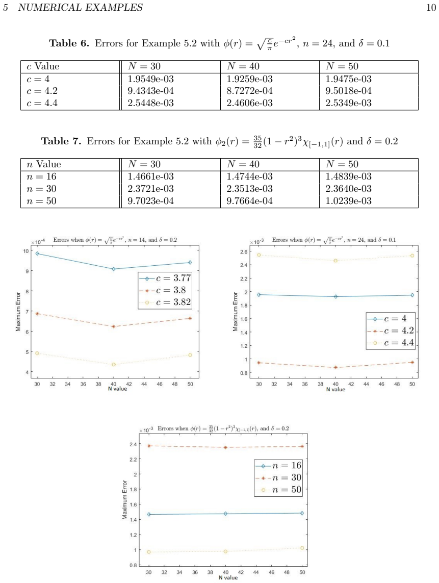
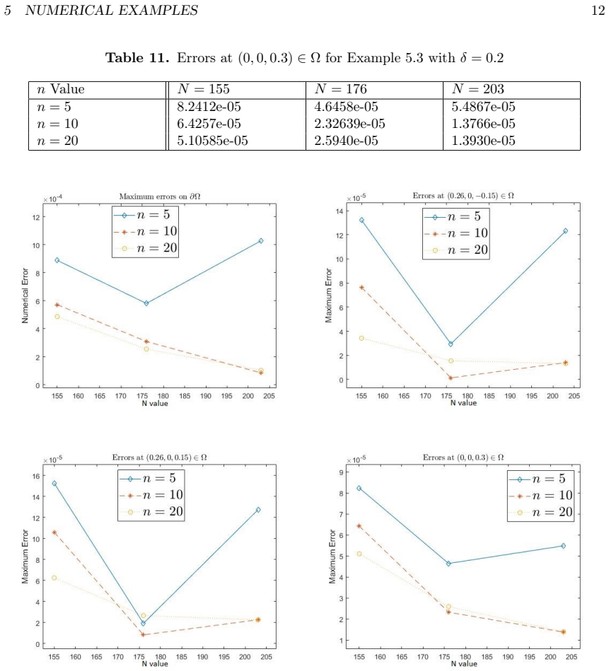
- In the worked examples the reported errors range roughly from $10^{-8}$ to $10^{-2}$ depending on the problem and parameters, suggesting the method is viable but its accuracy depends on the choice of RBF, $n$, $\delta$, and the number of boundary and source points.
Reading between the lines
- The paper does not describe how the improper integrals in (13) and (14) are evaluated; a natural next step is a careful quadrature and convergence study of these integrals, since their error propagates directly into every Helmholtz solve (this is the editor's inference, not a paper claim).
- The same reduction would apply to other time-dependent linear PDEs whose transform is a Helmholtz-type operator, such as the telegraph equation or damped wave equations.
- One testable extension is to replace the Gaussian and compactly supported RBFs used in the examples with other kernels and compare whether the accuracy plateaus; the formulas (13) and (14) are written for a general RBF $\phi$.
Editorial analysis
A structured set of objections, weighed in public.
Referee Report
Summary. The paper proposes a meshless method for diffusion and wave initial-boundary-value problems by converting them into sequences of Helmholtz boundary value problems, using either Laplace transforms or finite-difference time stepping, and solving each Helmholtz problem with a combination of the method of fundamental solutions (MFS) and the method of particular solutions (MPS). The particular solutions are taken from the integral representations of Li [9] rather than from RBF collocation. Numerical experiments cover homogeneous and non-homogeneous Helmholtz problems in two and three dimensions, a diffusion problem with very small diffusivity, and a vibrating membrane problem, with error tables comparing against analytical solutions.
Significance. If the derivations and numerical results were correct, the paper would offer a useful meshless alternative for time-dependent problems: it avoids meshing, uses the MFS for homogeneous parts, and replaces RBF collocation for particular solutions by the closed-sum approximations of [9]. The comparison against independent exact solutions in Examples 5.4-5.7 is a genuine strength, and the paper is not circular. However, several of the central algebraic transformations from the time-dependent PDEs to Helmholtz equations are incorrect as printed, and the numerical experiments therefore cannot be reproduced from the displayed equations. The paper also omits the quadrature details needed to evaluate the particular solutions in Eqs. (13)-(14), so its numerical claims are not independently checkable without code. The underlying idea is plausible, but the manuscript in its current form does not support the claimed conclusions.
major comments (4)
- [§4, Eqs. (30)-(35)] The backward Euler discretization of the diffusion equation (1/k)u_t = Δu is not what is written. With u_t(x,nτ) ≈ (u_n - u_{n-1})/τ, the correct implicit scheme is Δu_n - (1/(kτ))u_n = -(1/(kτ))u_{n-1}. Instead, Eq. (31) contains k(u_n-u_{n-1})/τ, and Eq. (34) becomes Δu_n - (k/τ)u_n = -(k/τ)u_{n-1} + ..., with λ = k/τ in Eq. (35). For k = 5.8e-7 in Example 5.5, this changes the Helmholtz coefficient by the factor k^2 ≈ 3.4e-13, so the scheme actually implemented cannot be the discretization of Eq. (45). This is a load-bearing error for the diffusion time-difference examples.
- [§3, Eq. (28) and §5, Example 5.6, Eq. (52)] The Laplace transform of the wave equation (1/c^2)u_tt = Δu is (s^2/c^2)U - (s/c^2)u_0 - (1/c^2)v_0 = ΔU. Eq. (28) is missing the factors 1/c^2 on the initial-condition terms. For Example 5.6, where c=1, u_0=0 and v_0=xy, the correct transformed equation is ΔU - s_l^2 U = -xy, but Eq. (52) has +xy on the right-hand side. This sign error changes the forcing term in every Helmholtz solve used for the reported wave results.
- [§5, Example 5.4, Eqs. (47)-(48)] The reduction from Eq. (45) to Eq. (47) is internally inconsistent. Since v = u - u_0 and u_0 = 1 is harmonic, v satisfies the same diffusion equation as u, namely (1/k)v_t = Δv, not v_t = Δv as printed in Eq. (47). Consequently, the Laplace-transformed Helmholtz problem should be ΔV - (s_l/k)V = 0, not ΔV - s_l V = 0 as in Eq. (48). For k = 5.8e-7 the coefficient s_l/k is roughly 1.72e6 times larger than s_l, so the example as written cannot reproduce the analytical solution (46), which explicitly contains k. This is a load-bearing inconsistency for the Laplace-transform diffusion example.
- [§2, Eqs. (13)-(14)] The approximate particular solutions un(x) are defined by sums of integrals over [0,∞) involving the RBF φ and Bessel/Hankel functions. The manuscript does not state how these infinite integrals are evaluated numerically, what quadrature is used, or what error control is imposed on the truncation. Since un(x) is added into every reported numerical solution through Eq. (17), an inaccurate or unstable evaluation of these integrals would invalidate all examples that use MPS. The paper provides no code, pseudocode, or implementation details, so this gap directly affects reproducibility of Tables 5-20.
minor comments (6)
- [General] The affiliation line contains a typo: "Portland State Univerisity" should be "Portland State University".
- [Eq. (25)] The left-hand side of Eq. (25) is written as eu(x,s), but the formula is an approximation to u(x,t) after inverse Laplace transformation; the argument should be t, not s.
- [Eq. (31)] Equation (31) introduces f(eun-1(x)) even though the diffusion equation (18) has no source term and the examples all set f = 0. The role of f in the time-difference formulation should be clarified or removed.
- [Eq. (36)] For the record, Eq. (36) is algebraically consistent with the central-difference discretization of (1/c^2)u_tt = Δu when c=1: moving the diagonal term to the left gives Δu_n - (1/(c^2τ^2))u_n = (u_{n-2} - 2u_{n-1})/(c^2τ^2), which matches the printed equation. No sign error appears there.
- [§5, Examples 5.4-5.7] The error tables report errors only at a small number of interior points and do not report convergence rates, condition numbers of the MFS linear systems, or dependence on the MFS source radius in the time-dependent examples. Such information would help the reader assess the reliability of the method.
- [Eq. (8)] The boundary condition in Eq. (8) is written with x ∈ Ω, but it should be x ∈ ∂Ω to describe a boundary condition.
Circularity Check
No significant circularity: the method is checked against independent exact solutions and its particular-solution component comes from an external, non-self citation.
full rationale
The claimed derivation chain is not circular. The paper takes approximate particular solutions un(x) for Helmholtz equations from the external reference [9] (Eqs. 13-14), solves the homogeneous residual problem by MFS (Eqs. 15-17), and then converts diffusion/wave IBVPs into sequences of Helmholtz BVPs by Laplace transform (Eqs. 21, 28) or time differences (Eqs. 34-36). No step defines an output in terms of itself: the approximate particular solution is not fitted to the paper's own numerical results, the MFS coefficients are determined by boundary residuals, and the reported errors are measured against analytic exact solutions (e.g., Eqs. 46, 51). The hyperparameter choices (c, δ, n, a, N) are tuning parameters, not data fitted to the predicted quantities. The paper contains no load-bearing self-citation: [9] is an independent prior work by another author. The substantive concerns are the unspecified quadrature for the infinite integrals in Eqs. (13)-(14) and apparent algebraic inconsistencies in the Laplace/time-difference discretizations (e.g., Eq. (48) versus the transform of Eq. (47), and Eq. (31) versus (35)). These are correctness and reproducibility risks, not circularity. Therefore the circularity score is 0.
Assumptions & free parameters
free parameters (6)
- Gaussian RBF width c =
e.g., 3.77, 3.8, 3.82 (Ex. 5.2); 0.1 (Ex. 5.3); 3 (Ex. 5.5); 10 (Ex. 5.6)
- Grid refinement n for particular solution =
e.g., 14, 16, 24, 50
- Domain padding delta =
0.1 or 0.2
- MFS source radius a =
5,6,7 (Ex. 5.1); 4 (Ex. 5.3); 2 (Ex. 5.4); 1.2 (Ex. 5.6-5.7)
- Stehfest parameter ns =
10 or 18
- Number of time steps M =
10, 15, 30
assumptions (5)
- domain assumption The approximate particular solution bound from [9]: ||un - u||_{C(Omega)} <= c/sqrt(n) ||f||_{C^1(Omega)} under mild conditions.
- domain assumption MFS converges for the homogeneous Helmholtz problem with analytic boundary data.
- domain assumption Stehfest inverse Laplace transform (25)-(26) yields an accurate approximation to the true inverse for the solutions considered.
- standard math Backward Euler and central difference schemes are stable for the diffusion and wave equations with the chosen tau.
- standard math The fundamental solution (9) is valid for complex kappa (modified Helmholtz cases).
Cite this review
Pith. "Pith review of Solving Diffusion and Wave Equations Meshlessly via Helmholtz Equations." pith.science (2026). https://pith.science/paper/RHB52XX5
@misc{pith2026241117122,
  author       = {Pith},
  title        = {Pith review of: Solving Diffusion and Wave Equations Meshlessly via Helmholtz Equations},
  year         = {2026},
  howpublished = {\url{https://pith.science/paper/RHB52XX5}},
  note         = {Machine review of arXiv:2411.17122}
}
read the original abstract
In this paper, using the approximate particular solutions of Helmholtz equations, we solve the boundary value problems of Helmholtz equations by combining the methods of fundamental solutions (MFS) with the methods of particular solutions (MPS). Then the initial boundary value problems of the time dependent diffusion and wave equations are discretized numerically into a sequence of Helmholtz equations with the appropriate boundary value conditions, which is done by either using the Laplace transform or by using time difference methods. Then Helmholtz problems are solved consequently in an iterative manner, which leads to the solutions of diffusion or wave equations. Several numerical examples are presented to show the efficiency of the proposed methods.
Figures


Figures from the paper (6 more)



Reference graph
Works this paper leans on
-
[9]
Approximation of potential integral by radial bases for solutions of Helmholtz equa- tion,
X. Li, "Approximation of potential integral by radial bases for solutions of Helmholtz equa- tion," Advances in Computational Mathematics , vol. 30, no. 3, pp. 201-230, 2009, Springer
work page 2009
-
[1]
The Method of Fundamental Solutions for Potential, Helmholtz andDiffusionProblems,
M.A. Golberg and C.S. Chen, "The Method of Fundamental Solutions for Potential, Helmholtz andDiffusionProblems,"in Boundary Integral Methods: Numerical and Mathematical Aspects, vol. 1, WIT press Southampton, 1998, pp. 103-176
work page 1998
-
[2]
Radial Basis Approximation for Newtonian Potentials,
X. Li, "Radial Basis Approximation for Newtonian Potentials,"Advances in Computational Mathematics, vol. 33, no. 1, 2010. REFERENCES 18
work page 2010
-
[3]
Convergence of the Method of Fundamental Solutions for Poisson’s Equation on the Unit Sphere,
X. Li, "Convergence of the Method of Fundamental Solutions for Poisson’s Equation on the Unit Sphere," Advances in Computational Mathematics , vol. 28, no. 3, pp. 269-282, 2008, Springer
work page 2008
-
[4]
The method of fundamental solutions for elliptic bound- ary value problems,
G. Fairweather and A. Karageorghis, "The method of fundamental solutions for elliptic bound- ary value problems,"Advances in Computational Mathematics , vol. 9, no. 1, pp. 69-95, 1998, Springer
work page 1998
-
[5]
M. Choi, "Meshless Methods for Numerically Solving Boundary Value Problems of Elliptic Type Partial Differential Equations," Ph.D. dissertation, UNLV, 2018
work page 2018
-
[6]
Solving linear diffusion equations with the dual reciprocity method in Laplace space,
S. Zhu, P. Satravaha, and X. Lu, "Solving linear diffusion equations with the dual reciprocity method in Laplace space,"Engineering Analysis with Boundary Elements , vol. 13, no. 1, pp. 1-10, 1994, Elsevier
work page 1994
-
[7]
The Laplace transform boundary element (LTBE) method for the solution of diffusion-type equations,
G.J. Moridis and D.L. Reddel, "The Laplace transform boundary element (LTBE) method for the solution of diffusion-type equations," inBoundary Elements XIII , pp. 83-97, Springer, 1991
work page 1991
Show all 21 references
-
[8]
Algorithm 368: Numerical inversion of Laplace transforms [D5],
H. Stehfest, "Algorithm 368: Numerical inversion of Laplace transforms [D5],"Communica- tions of the ACM , vol. 13, no. 1, pp. 47-49, 1970, ACM New York, NY, USA
1970
-
[10]
The method of fundamental solutions for the Helmholtz equation,
Z.C. Li, Y. Wei, Y. Chen, and H.T. Huang, "The method of fundamental solutions for the Helmholtz equation," Applied Numerical Mathematics, vol. 135, pp. 510-536, 2019, Elsevier
2019
-
[11]
Solutions of 2D and 3D Stokes laws using multiquadrics method,
D.L. Young, S.C. Jane, C.Y. Lin, C.L. Chiu, and K.C. Chen, "Solutions of 2D and 3D Stokes laws using multiquadrics method,"Engineering Analysis with Boundary Elements , vol. 28, no. 10, pp. 1233-1243, 2004, Elsevier
2004
-
[12]
Ameshlesssolutiontotwo-dimensionalconvection–diffusionproblems,
V.PopovandT.Bui, "Ameshlesssolutiontotwo-dimensionalconvection–diffusionproblems," Engineering Analysis with Boundary Elements , vol. 34, no. 7, pp. 680-689, 2010, Elsevier
2010
-
[13]
Fast Solution for Solving the Modified Helmholtz Equation with the Method of Fundamental Solutions,
C.S. Chen, X. Jiang, W. Chen, and G. Yao, "Fast Solution for Solving the Modified Helmholtz Equation with the Method of Fundamental Solutions,"Communications in Computational Physics, vol. 17, no. 3, pp. 867-886, 2015, Cambridge University Press
2015
-
[14]
A survey of applications of the MFS to inverse problems,
A. Karageorghis, D. Lesnic, and L. Marin, "A survey of applications of the MFS to inverse problems," Inverse Problems in Science and Engineering , vol. 19, no. 3, pp. 309-336, 2011, Taylor & Francis
2011
-
[15]
Radial basis approximation and its application to biharmonic equation,
X. Li, "Radial basis approximation and its application to biharmonic equation,"Advances in Computational Mathematics, vol. 32, no. 3, pp. 275-302, 2010, Springer
2010
-
[16]
A novel RBF collocation method using fictitious centres,
C.S. Chen, A. Karageorghis, and F. Dou, "A novel RBF collocation method using fictitious centres," Applied Mathematics Letters, vol. 101, p. 106069, 2020, Elsevier
2020
-
[17]
A fictitious points one–step MPS–MFS technique,
X. Zhu, F. Dou, A. Karageorghis, and C.S. Chen, "A fictitious points one–step MPS–MFS technique," Applied Mathematics and Computation , vol. 382, p. 125332, 2020, Elsevier
2020
-
[18]
Improved Kansa RBF method for the so- lution of nonlinear boundary value problems,
M.A. Jankowska, A. Karageorghis, and C.S. Chen, "Improved Kansa RBF method for the so- lution of nonlinear boundary value problems,"Engineering Analysis with Boundary Elements , vol. 87, pp. 173-183, 2018, Elsevier
2018
-
[19]
Radial basis function approximation in the dual reci- procity method,
S.R. Karur and P.A. Ramachandra, "Radial basis function approximation in the dual reci- procity method," Mathematical and Computer Modelling , vol. 20, no. 7, pp. 59-70, 1994, Elsevier
1994
-
[20]
Analytic Particular Solutions for Inhomogeneous Helmholtz-Type Equations,
A.S. Muleshkov, C.S. Chen, M.A. Golberg, and A.H.-D. Cheng, "Analytic Particular Solutions for Inhomogeneous Helmholtz-Type Equations," Advances in Computational Engineering & Sciences, vol. 1, pp. 27-32, 2000, Tech Science Press. REFERENCES 19
2000
-
[21]
Lecture Note Laplace Transform for Solving Linear Diffusion Equations
C.S. Chen, "Lecture Note Laplace Transform for Solving Linear Diffusion Equations."
Reviewed August 12, 2026 · model on record in the stance chip above.
Discussion (0). Continue with ORCID to comment.