REVIEW 3 major objections 7 minor 39 references
Multiscale Jones Polynomial and Persistent Jones Polynomial for Knot Data Analysis
T0 review · 3 major / 7 minor · reviewed 2026-08-12 · deepseek-v4-flash
Pith's one-line read The Jones polynomial can be localized to open curve segments with proven stability bounds.
desk verdict New localized Jones-polynomial descriptors look useful, but the persistence-stability theorem rests on a false premise and an unproved lemma; worth refereeing only if the stability proofs are fixed. read the letter →
The pith
A machine-rendered reading of the paper's core claim, the machinery that carries it, and where it could break.
The reading
What carries the argument
Two objects carry the argument. The first is the evaluation map $t\mapsto J(10)$ applied to the projection-averaged Jones polynomial of curve collections, which turns a polynomial invariant into a real-valued continuous function of the curve coordinates; this gives the bound $\epsilon_J$. The second is the facet barcode of a Vietoris-Rips filtration, the nested family of simplicial complexes built by connecting curve segments whose pairwise distances fall below a growing threshold; maximal simplices, or facets, are born and die as the threshold grows, and each facet is assigned the Jones polynomial of the corresponding curve segments as a weight. The stability proof couples these with a box-counting lemma from persistence-diagram theory, which bounds the number of points that a shifted diagram can place in a shrunk box, and with a matching argument that pairs each facet of the original diagram to a facet of the perturbed diagram.
What would settle it
Search over small configurations of three or four short curve segments: perturb one segment by a sup-norm shift of size $\epsilon$, compute the two weighted facet diagrams of the persistent Jones polynomial at $t=10$, and compare them with the weighted bottleneck distance. If any example gives a distance larger than $\max\{2\epsilon,\epsilon_J\}$, the theorem's bound is false. A simpler diagnostic is to find a configuration in which a facet dies at $y$ although one outside segment lies closer than $y$ to one facet member and another lies farther than $y$, which would contradict the proof's all-outside-segments distance premise.
Extended reading notes
Core claim
On the paper's own terms, the discovery is that the Jones polynomial, a topological invariant that is normally defined for closed knots, can be localized to the scale of curve segments while retaining a controlled response to perturbation. Given a segmentation $P_n=\{l_1,\dots,l_n\}$ of a curve collection $L$, the multiscale model forms, for every segment $l_i$ and every distance window $[r,R)$, the set of segments within that window and evaluates the Jones polynomial of that subset at $t=10$. The persistent model filters the segments by the Vietoris-Rips complex and records the birth and death of each maximal simplex (facet), weighting the point $(x,y)$ in the resulting diagram by the Jones polynomial, again at $t=10$, of the segments that form the facet. Theorem 4.1 and Theorem 4.2 assert that both models are stable: under a continuous map $f$ with $\|f(L)-L\|_\infty<\epsilon$, the matrix entries move by less than $\epsilon_J$, and the weighted bottleneck distance between the diagrams is less than $\max\{2\epsilon,\epsilon_J\}$.
Load-bearing premise
The persistent stability proof assumes that a facet dies only when every outside segment is at least the death distance from every inside segment, whereas the Vietoris-Rips complex only guarantees this for some inside segment per outside segment; if that stronger distance condition fails, the diagram-matching argument in Section 4.2.2 has no support.
Editorial extensions
If this is right
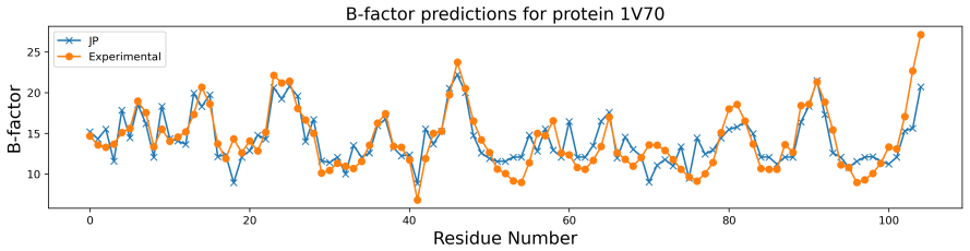
- The multiscale Jones polynomial yields a real-valued characteristic matrix for any segmented curve collection, so it can be fed directly into regression or machine-learning models; the paper reports B-factor correlations of $0.899$, $0.808$, and $0.720$ on small, medium, and large protein sets.
- The persistent Jones polynomial produces weighted barcodes that distinguish protein secondary structures; the reported $\alpha$-helix weights span $-86$ to $0$ while the $\beta$-sheet weights span $-6$ to $0$.
- The stability bounds imply that feature vectors built from either model are insensitive to small geometric noise, provided the segmentation and distance windows are held fixed.
- Both models reduce to global knot information when a segment covers the whole curve and to trivial local information when segments are very short, so segmentation length is a tunable resolution parameter.
Reading between the lines
- Editorial extension: the same segmentation-and-weighting construction could be applied to other knot polynomial invariants that vary continuously under small curve moves, giving analogous multiscale and persistent descriptors with their own stability bounds.
- Editorial extension: because the facet barcodes track maximal simplices rather than homology classes, the paper opens a separate stability question for facet persistence itself; a matching lemma proved directly for Vietoris-Rips facets would either repair or replace the imported counting lemma.
- Editorial extension: the evaluation point $t=10$ is a modeling choice; evaluating at several values of $t$ and concatenating the resulting matrices or diagrams would likely produce richer features without changing the stability argument.
Editorial analysis
A structured set of objections, weighed in public.
Referee Report
Summary. The paper proposes two localizations of the Jones polynomial for collections of disjoint open or closed curves in R^3, building on the averaged bracket polynomial of Barkataki and Panagiotou [5]. The multiscale Jones polynomial is an n x m matrix of evaluations at t=10, where each entry is the Jones polynomial of the set of segments within a distance window [r,R) of a given segment. The persistent Jones polynomial is defined by weighting the facets of a Vietoris-Rips filtration of the segmentation by the Jones polynomial of the corresponding curve segments, yielding weighted barcodes and weighted persistence diagrams. Section 4 claims stability: Theorem 4.1 states that the multiscale characteristic matrix changes by less than epsilon_J under a sup-norm perturbation of size epsilon, and Theorem 4.2 states that the weighted bottleneck distance between persistent Jones diagrams is less than max{2 epsilon, epsilon_J}. Section 5 applies the multiscale model to B-factor prediction and the persistent model to alpha-helix and beta-sheet barcodes.
Significance. If the stability theorems were valid, the paper would provide a useful new class of localized, stable knot-theoretic descriptors for curve data, extending the mGLI approach [35] and the weighted-barcode idea [8] to the Jones polynomial. The novelty lies in replacing global knot invariants with scale-dependent and persistence-based versions and in the reported B-factor correlation coefficients. The manuscript should be credited for building on prior definitions rather than inventing ad hoc entities. However, the theoretical contribution is the central claim, and it is not established: Theorem 4.2 relies on an unproved Box Lemma and a false death-time statement, and Theorem 4.1 relies on an unjustified boundary-separation step. The application results, while suggestive, are presented without statistical detail. Thus the paper cannot be accepted in its current form.
major comments (3)
- [§4.2.2, Lemma 4.1] Lemma 4.1 is imported from Cohen-Steiner-Edelsbrunner-Harer [9], but that result applies to persistence diagrams arising from homology persistence modules. Here the diagram D(Pn) is built from facets of a Vietoris-Rips filtration, and the quantity beta^y_x is a facet count, not a homology rank. No proof is given that the Box-Lemma inequality #(D(Pn) intersect R_{2 epsilon}) <= #(D(f(Pn)) intersect R) holds for these facet diagrams. Every counting step in the proof of Theorem 4.2 (the inequalities mu <= #(...), the equality #(...)=mu, and the exclusion of unmatched points) depends on this lemma. The persistent stability bound is therefore unsupported as written.
- [§4.2.2, death condition in Theorem 4.2] The proof of Theorem 4.2 states that if a facet Pn(p) dies at y, then any segment l outside Pn(p) is at distance at least y from every segment in Pn(p). In the Vietoris-Rips filtration this is false: a facet dies at the infimum over outside vertices of their maximum distance to the facet's vertices, so for each outside segment it is only guaranteed that some vertex of the facet is at distance at least y, not all. The lower bound on the death of the image facet under f is therefore not justified by the stated hypothesis. The proof also does not justify the upper bound 'death <= y'; under a perturbation the death time can increase by up to 2 epsilon. These issues affect the claimed bound ||f(p)-p||_infinity < 2 epsilon and the matching argument.
- [§4.1, Proposition 4.1] The proof of Proposition 4.1 concludes P^i_{r-4 epsilon, R+4 epsilon} = P^i_{r,R} from smallness of epsilon. This equality is false without a separation condition: if some distance d(l_i,l_j) equals r or R, or lies within 4 epsilon of the boundary, a perturbation of size < epsilon can move the distance across the boundary and change membership of the segment. Theorem 4.1, which relies on this equality to identify f(P^i_{r,R}) with f(P)^i_{r,R}, therefore does not follow from the hypotheses as stated. A non-degeneracy condition on the distance matrix relative to the radius parameters, or a reformulation of the stability statement, is needed.
minor comments (7)
- [Title] The title in the full text reads 'Multisacle Jones Polynomial'; the typo should be corrected.
- [§3.1] The distance d(l_i,l_j) is described as 'the upper bound of the Eulerian distances'; it should be explicitly defined as sup_{x in l_i, y in l_j} |x-y| to avoid ambiguity.
- [§4.2] The multiplicity mu^i_j is defined for a 'fixed integer k' without first specifying the range of facet dimensions; the dependence of D(Pn) on k should be stated.
- [§4.2.1] The weighted bottleneck distance treats diagonal points as having infinite multiplicity in the diagrams, but the matching definition for multi-sets of pairs does not specify how diagonal points are handled; the diagonal convention should be made explicit.
- [§5.1] The reported correlation coefficients (0.899, 0.808, 0.720) are averages across protein sets, but no error bars, number of proteins per set, or statistical comparison with the listed baselines is provided.
- [§5.2] The statement that 'a greater color difference between two bars suggests a greater difference between the sets of curve segments they represent' is not a quantitative claim; the color scale is the Jones polynomial weight and the relation to entanglement complexity is unexplained.
- [§4.2.2] The final sentence of Section 4.2.2 says the diagrams are stable under 'possibly irregular perturbations'; the term 'irregular' is not defined in the paper.
Circularity Check
No significant circularity: the stability claims are derived from the externally quoted continuity of the open-curve Jones polynomial and from explicit perturbation bounds, not from the conclusions being proved; the cited Box Lemma and the facet-death condition are correctness gaps, not circular reductions.
full rationale
The derivation chain for Theorem 4.1 begins with Proposition 2.1, quoted from [5], that the open-curve Jones polynomial is a continuous function of the curve coordinates, and then bounds each characteristic-matrix entry by |J_{P^i}(10) - J_{f(P^i)}(10)| < ε_J together with the segment-set equality of Proposition 4.1. This is a direct input-to-output estimate, not a restatement of the theorem. The persistent stability theorem is likewise assembled from explicit bounds: births move by at most 2ε via the Rips distance inequality, deaths are claimed to move by at most 2ε, and weights move by at most ε_J by the same continuity result, so the bottleneck bound max{2ε, ε_J} follows from the constructed matching. No fitted parameter is renamed as a prediction, and the target inequality is not assumed among the hypotheses. The main weaknesses are mathematical rather than circular: Lemma 4.1 from [9] is a homology persistence-diagram statement and the manuscript supplies no proof that the facet-based diagrams satisfy it, and the assertion in Section 4.2.2 that an outside segment is at distance at least y from every segment of the facet is stronger than the Rips death condition, which only requires the maximum distance over the facet to be at least y for each outside segment. These are unproved-step and correctness risks that a referee should ask the authors to repair, but they do not make the theorem definitionally equivalent to its input. The self-citations to [35] and [8] are contextual or comparative: the mGLI model is used as a benchmark, and the weighted barcode is used as a representational device; neither supplies the stability bound. Hence the paper is not circular.
Assumptions & free parameters
free parameters (5)
- Jones polynomial evaluation point =
t = 10
- Distance window radii r and R =
r in [4,15] Angstrom step 0.25; R = r+1 Angstrom
- Lasso regularization parameter =
0.16
- Segmentation P_n =
cut at midpoints between consecutive C-alpha atoms
- Distance between segments =
distance between C-alpha atoms within segments
assumptions (5)
- domain assumption The open-curve Jones polynomial from [5] is well-defined, has real coefficients, and is continuous in the curve coordinates.
- ad hoc to paper The Cohen-Steiner-Edelsbrunner-Harer Box Lemma applies to the facet-based persistence diagrams defined in Section 3.2.
- ad hoc to paper For a facet that dies at y, every outside segment is at distance at least y from every segment in the facet.
- standard math Perturbing each point by at most epsilon changes any pairwise distance by at most 2 epsilon.
- standard math A finite Vietoris-Rips filtration has finitely many critical values and its final complex is an (n-1)-simplex.
Cite this review
Pith. "Pith review of Multiscale Jones Polynomial and Persistent Jones Polynomial for Knot Data Analysis." pith.science (2026). https://pith.science/paper/PLDMFZKJ
@misc{pith2026241117331,
  author       = {Pith},
  title        = {Pith review of: Multiscale Jones Polynomial and Persistent Jones Polynomial for Knot Data Analysis},
  year         = {2026},
  howpublished = {\url{https://pith.science/paper/PLDMFZKJ}},
  note         = {Machine review of arXiv:2411.17331}
}
read the original abstract
Many structures in science, engineering, and art can be viewed as curves in 3-space. The entanglement of these curves plays a crucial role in determining the functionality and physical properties of materials. Many concepts in knot theory provide theoretical tools to explore the complexity and entanglement of curves in 3-space. However, classical knot theory primarily focuses on global topological properties and lacks the consideration of local structural information, which is critical in practical applications. In this work, two localized models based on the Jones polynomial, namely the multiscale Jones polynomial and the persistent Jones polynomial, are proposed. The stability of these models, especially the insensitivity of the multiscale and persistent Jones polynomial models to small perturbations in curve collections, is analyzed, thus ensuring their robustness for real-world applications.
Figures


Figures from the paper (6 more)




Reference graph
Works this paper leans on
-
[5]
Kasturi Barkataki and Eleni Panagiotou. The jones polynomial of collections of open curves in 3-space.Proceedings of the Royal Society A, 478(2267):20220302, 2022
work page 2022
-
[35]
Li Shen, Hongsong Feng, Fengling Li, Fengchun Lei, Jie Wu, and Guo-Wei Wei. Knot data analysis using multiscale gauss link integral.Proceedings of the National Academy of Sciences, 121(42):e2408431121, 2024
work page 2024
-
[8]
Persistent cohomology for data with multicomponent heterogeneous information
Zixuan Cang and Guo-Wei Wei. Persistent cohomology for data with multicomponent heterogeneous information. SIAM journal on mathematics of data science, 2(2):396–418, 2020
work page 2020
-
[9]
Stability of persistence diagrams
David Cohen-Steiner, Herbert Edelsbrunner, and John Harer. Stability of persistence diagrams. InProceedings of the twenty-first annual symposium on Computational geometry, pages 263–271, 2005
work page 2005
-
[1]
Alexander and W. J. Topological invariants of knots and links. Transactions of the American Mathematical Society, 30(2):275–306, 1928. 24
work page 1928
-
[2]
Javier Arsuaga, Mariel Vazquez, Paul McGuirk, Sonia Trigueros, De Witt Sumners, and Joaquim Roca. Dna knots reveal a chiral organization of dna in phage capsids.Proceedings of the National Academy of Sciences, 102(26):9165–9169, 2005
work page 2005
-
[3]
The local topological free energy of proteins
Quenisha Baldwin and Eleni Panagiotou. The local topological free energy of proteins. Journal of Theoretical Biology, 529:110854, 2021
work page 2021
-
[4]
The local topological free energy of the sars-cov-2 spike protein.Polymers, 14(15):3014, 2022
Quenisha Baldwin, Bobby Sumpter, and Eleni Panagiotou. The local topological free energy of the sars-cov-2 spike protein.Polymers, 14(15):3014, 2022
work page 2022
Show all 39 references
-
[6]
Atom-specific persistent homology and its application to protein flexibility analysis.Computational and mathematical biophysics, 8(1):1–35, 2020
David Bramer and Guo-Wei Wei. Atom-specific persistent homology and its application to protein flexibility analysis.Computational and mathematical biophysics, 8(1):1–35, 2020
2020
-
[7]
Evolutionary homology on coupled dynamical systems with applications to protein flexibility analysis.Journal of applied and computational topology, 4:481–507, 2020
Zixuan Cang, Elizabeth Munch, and Guo-Wei Wei. Evolutionary homology on coupled dynamical systems with applications to protein flexibility analysis.Journal of applied and computational topology, 4:481–507, 2020
2020
-
[10]
Introduction to knot theory, volume 57
Richard H Crowell and Ralph Hartzler Fox. Introduction to knot theory, volume 57. Springer Science & Business Media, 2012
2012
-
[11]
A new polynomial invariant of knots and links
Peter Freyd, David Yetter, Jim Hoste, WB Raymond Lickorish, Kenneth Millett, and Adrian Ocneanu. A new polynomial invariant of knots and links. 1985
1985
-
[12]
Parity in knotoids
Neslihan G¨ ug¨ umc¨ u and Louis Kauffman. Parity in knotoids. arXiv preprint arXiv:1905.04089, 2019
1905 arXiv
-
[13]
New invariants of knotoids.European Journal of Combinatorics, 65:186–229, 2017
Neslihan G¨ ug¨ umc¨ u and Louis H Kauffman. New invariants of knotoids.European Journal of Combinatorics, 65:186–229, 2017
2017
-
[14]
Knotoids, braidoids and applications
Neslihan G¨ ug¨ umc¨ u and Sofia Lambropoulou. Knotoids, braidoids and applications. Symmetry, 9(12):315, 2017. 25
2017
-
[15]
A computational package for measuring topological entanglement in polymers, proteins and periodic systems (teppp)
Tom Herschberg, Kyle Pifer, and Eleni Panagiotou. A computational package for measuring topological entanglement in polymers, proteins and periodic systems (teppp). Computer Physics Communications, 286:108639, 2023
2023
-
[16]
Jones and F. R. Vaughan. A polynomial invariant for knots via von neumann algebras. Bulletin of the American Mathematical Society, 12(1):103–111, 1985
1985
-
[17]
An invariant of regular isotopy
Louis H Kauffman. An invariant of regular isotopy. Transactions of the American Mathematical Society, 318(2):417–471, 1990
1990
-
[18]
A categorification of the jones polynomial
Mikhail Khovanov. A categorification of the jones polynomial. 2000
2000
-
[19]
Knots in proteins.Journal of the American Chemical Society, 116(24):11189–11190, 1994
Chengzhi Liang and Kurt Mislow. Knots in proteins.Journal of the American Chemical Society, 116(24):11189–11190, 1994
1994
-
[20]
The geometry of periodic knots, polycatenanes and weaving from a chemical perspective: a library for reticular chemistry.Chemical Society Reviews, 47(12):4642–4664, 2018
Yuzhong Liu, Michael O’Keeffe, Michael MJ Treacy, and Omar M Yaghi. The geometry of periodic knots, polycatenanes and weaving from a chemical perspective: a library for reticular chemistry.Chemical Society Reviews, 47(12):4642–4664, 2018
2018
-
[21]
An introduction to knot floer homology.Physics and mathematics of link homology, 680:99–135, 2016
Ciprian Manolescu. An introduction to knot floer homology.Physics and mathematics of link homology, 680:99–135, 2016
2016
-
[22]
Finite type invariants for knotoids
Manousos Manouras, Sofia Lambropoulou, and Louis H Kauffman. Finite type invariants for knotoids. European Journal of Combinatorics, 98:103402, 2021
2021
-
[23]
Identifying knots in proteins.Biochemical Society Transactions, 41(2):533–537, 2013
Kenneth C Millett, Eric J Rawdon, Andrzej Stasiak, and Joanna I Su lkowska. Identifying knots in proteins.Biochemical Society Transactions, 41(2):533–537, 2013
2013
-
[24]
Quantum invariants: A study of knots, 3-manifolds, and their sets, volume 29
Tomotada Ohtsuki. Quantum invariants: A study of knots, 3-manifolds, and their sets, volume 29. World Scientific, 2002
2002
-
[25]
Fast and anisotropic flexibility-rigidity index for protein flexibility and fluctuation analysis
Kristopher Opron, Kelin Xia, and Guo-Wei Wei. Fast and anisotropic flexibility-rigidity index for protein flexibility and fluctuation analysis. The Journal of chemical physics, 140(23), 2014
2014
-
[26]
Knot polynomials of open and closed curves
Eleni Panagiotou and Louis H Kauffman. Knot polynomials of open and closed curves. Proceedings of the Royal Society A, 476(2240):20200124, 2020
2020
-
[27]
Vassiliev measures of complexity of open and closed curves in 3-space.Proceedings of the Royal Society A, 477(2254):20210440, 2021
Eleni Panagiotou and Louis H Kauffman. Vassiliev measures of complexity of open and closed curves in 3-space.Proceedings of the Royal Society A, 477(2254):20210440, 2021
2021
-
[28]
Topological methods for polymeric materials: characterizing the relationship between polymer entanglement and viscoelasticity
Eleni Panagiotou, Kenneth C Millett, and Paul J Atzberger. Topological methods for polymeric materials: characterizing the relationship between polymer entanglement and viscoelasticity. Polymers, 11(3):437, 2019. 26
2019
-
[29]
A topological study of protein folding kinetics
Eleni Panagiotou and Kevin W Plaxco. A topological study of protein folding kinetics. Topol. Geom. Biopolym. AMS Contemp. Math. Ser, 746:223–233, 2020
2020
-
[30]
Coarse grained normal mode analysis vs
Jun-Koo Park, Robert Jernigan, and Zhijun Wu. Coarse grained normal mode analysis vs. refined gaussian network model for protein residue-level structural fluctuations.Bulletin of mathematical biology, 75:124–160, 2013
2013
-
[31]
Conway algebras and skein equivalence of links
J´ ozef H Przytycki and Pawel Traczyk. Conway algebras and skein equivalence of links. Proceedings of the American Mathematical Society, pages 744–748, 1987
1987
-
[32]
Counting polymer knots to find the entanglement length
Jian Qin and Scott T Milner. Counting polymer knots to find the entanglement length. Soft Matter, 7(22):10676–10693, 2011
2011
-
[33]
Topology bounds energy of knots and links
Renzo L Ricca. Topology bounds energy of knots and links. Proceedings of the Royal Society A: Mathematical, Physical and Engineering Sciences, 464(2090):293–300, 2008
2008
-
[34]
To knot or not to knot: multiple conformations of the sars-cov-2 frameshifting rna element
Tamar Schlick, Qiyao Zhu, Abhishek Dey, Swati Jain, Shuting Yan, and Alain Laederach. To knot or not to knot: multiple conformations of the sars-cov-2 frameshifting rna element. Journal of the American Chemical Society, 143(30):11404–11422, 2021
2021
-
[36]
Conservation of complex knotting and slipknotting patterns in proteins
Joanna I Sulkowska, Eric J Rawdon, Kenneth C Millet, Jose N Onuchic, and Andrzej Stasiak. Conservation of complex knotting and slipknotting patterns in proteins. Biophysical Journal, 102(3):253a, 2012
2012
-
[37]
The role of knot theory in dna research
DW Sumners. The role of knot theory in dna research. InGeometry and Topology, pages 297–318. CRC Press, 2020
2020
-
[38]
Knotoids.Osaka Journal of Mathematics, 49(1):195–223, 2012
Vladimir Turaev. Knotoids.Osaka Journal of Mathematics, 49(1):195–223, 2012
2012
-
[39]
The protein folding rate and the geometry and topology of the native state.Scientific Reports, 12(1):6384, 2022
Jason Wang and Eleni Panagiotou. The protein folding rate and the geometry and topology of the native state.Scientific Reports, 12(1):6384, 2022. 27
2022
Reviewed August 12, 2026 · model on record in the stance chip above.
Discussion (0). Continue with ORCID to comment.