pith. sign in

arxiv: 2411.17509 · v2 · submitted 2024-11-26 · 🧮 math.SG · math.DS· nlin.SI

On the affine invariant of simple hypersemitoric systems

Pith reviewed 2026-05-23 17:31 UTC · model grok-4.3

classification 🧮 math.SG math.DSnlin.SI
keywords hypersemitoric systemsaffine invariantDelzant polytopesemitoric systemsintegrable systemssymplectic manifoldsHamiltonian circle actionsmoment maps
0
0 comments X

The pith

Hypersemitoric systems possess an affine invariant that generalizes the Delzant polytope of toric systems and the polytope invariant of semitoric systems.

A machine-rendered reading of the paper's core claim, the machinery that carries it, and where it could break.

The paper introduces an affine invariant for hypersemitoric systems, a class of integrable systems on four-dimensional symplectic manifolds that feature only mildly degenerate singularities and include one proper effective Hamiltonian circle action. This invariant extends the combinatorial descriptions already available for the toric and semitoric cases, so that the same object can be attached to a broader family of systems. The authors also compute the invariant explicitly on a sequence of concrete examples that grow in complexity. A sympathetic reader would therefore see a single, uniform tool for recording the global structure of these systems instead of separate constructions for each subclass.

Core claim

We introduce the affine invariant of hypersemitoric systems, which is a generalization of the Delzant polytope of toric systems and the polytope invariant of semitoric systems. Along the way, we compute and plot this invariant for meaningful and more and more complicated examples.

What carries the argument

The affine invariant, an object that records the image of the moment map together with an affine structure on the base space, extending the polytope constructions used for toric and semitoric systems.

If this is right

  • The same invariant applies uniformly to toric, semitoric, and hypersemitoric systems.
  • Explicit computations become feasible for successively more complicated examples.
  • The invariant supplies a combinatorial object that can be plotted and compared across the whole class.
  • Classification questions for hypersemitoric systems can now be phrased in terms of this single affine object.

Where Pith is reading between the lines

These are editorial extensions of the paper, not claims the author makes directly.

  • The construction may allow direct comparison between hypersemitoric systems and other integrable systems whose singularities lie outside the current definition.
  • One could test whether the invariant remains unchanged under small deformations that preserve the hypersemitoric conditions.
  • The existence of the invariant suggests that a global classification of hypersemitoric systems up to isomorphism might be possible by enumerating admissible affine images.
  • If the invariant distinguishes non-isomorphic systems, it could be used to decide whether two given hypersemitoric systems are equivalent.

Load-bearing premise

That hypersemitoric systems, defined by their mild degeneracies and the existence of a proper effective circle action, admit a well-defined affine invariant that matches the earlier polytopes on the toric and semitoric subcases without extra consistency requirements.

What would settle it

A concrete hypersemitoric system whose moment-map image cannot be equipped with a consistent affine structure that reduces to the known Delzant or semitoric polytope when the system is toric or semitoric.

Figures

Figures reproduced from arXiv: 2411.17509 by Konstantinos Efstathiou, Pedro Santos, Sonja Hohloch.

Figure 2.1
Figure 2.1. Figure 2.1: Example of a standard flap with one elliptic-elliptic value represented in the black dot. The red line represents the hyperbolic-regular values in the flap. The green points correspond to the parabolic values in the flap. Then blue lines represent the elliptic-regular values in the flap. 2.13. Local normal form and isotropy weights of an S 1 -action. Definition 2.18. A Hamiltonian S 1 -space is a triple … view at source ↗
Figure 2.2
Figure 2.2. Figure 2.2: Example of a pleat. The red line represents the hyperbolic￾regular values in the pleat. The green dots correspond to the parabolic values of the pleat. The blue lines represent the elliptic-regular values. (U, ω) (U0, ω0) R J Ψ J0 We refer to the integers n, m in Lemma 2.19 as the isotropy weights of J at p. If the action is effective the integers n, m are coprime. 2.14. Monodromy in the presence of an S… view at source ↗
Figure 3.1
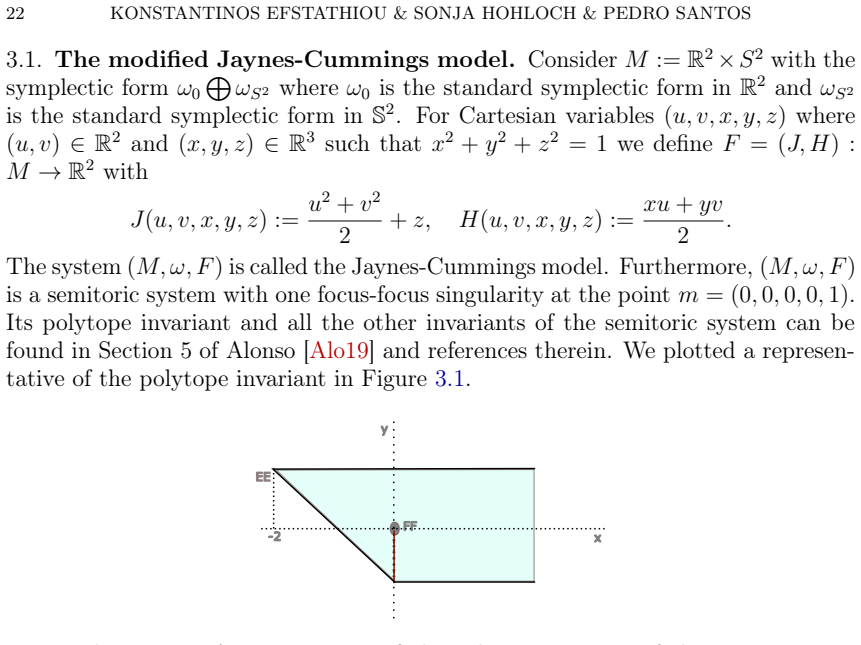
Figure 3.1. Figure 3.1: A representative of the polytope invariant of the Jaynes￾Cummings model for ϵ = −1. The point labeled F F is the focus-focus value and the point labeled by EE is the elliptic-elliptic value of the sys￾tem. The red line represents the cut associated with the choice of ϵ. Dullin & Pelayo [DP16] considered the system (M, ω, F = (J, H + G)) where the function G is given by G(u, v, x, y, z) = γz2 with γ = 4 5… view at source ↗
Figure 3.2
Figure 3.2. Figure 3.2: The bifurcation diagram for the system (J, ω,(J, H + G)). The red dot represents the elliptic-elliptic value on the flap. Proposition 3.3. Let (M, ω, F = (J, H)) be a hypersemitoric system and F a flap. Then the boundary of F consists of two parabolic values joined by two types of curves in the following way: one curve consists only of hyperbolic-regular values. The other curve consists of elliptic-regul… view at source ↗
Figure 4.1
Figure 4.1. Figure 4.1: The joint spectrum of (J, H + G) when ℏ = 2 101 . The green dots correspond to values outside of the flap. The red dots correspond to values on the background of the flap. The blue dots correspond to values on the flappy part of the flap, but they are barely visible since they overlap mostly with the red dots. of Wα,β,n as the symplectic reduction of C 4 . The quantization of C 4 is the Hilbert space L 2… view at source ↗
Figure 4.2
Figure 4.2. Figure 4.2: The joint spectrum of (J = |z2| 2 2 , R = |z3| 2 2 ) for ℏ = 0.05 and α = β = n = 1. 5. Affine invariant in the presence of a standard flap 5.1. Intuition. Recall that when a system admits a standard flap the set of regular values is not simply connected and the system displays monodromy due to the presence of elliptic-elliptic values, see Proposition 2.20. There are two ways to deal with this phenomenon… view at source ↗
Figure 5.1
Figure 5.1. Figure 5.1: Rule that the paths used in Theorem 5.1 in order to define action-angle coordinates need to follow in the case n = 2 and ⃗ϵ = (1, 1). of the elliptic critical values in the boundary of F(M) are caused by standard flaps Fi , i = 1, ..., n. Let ci be the points defined in Section 5.2. Note that by Corollary 5.6, it follows that n < ∞. For ⃗ϵ ∈ {−1, 1} n , Theorem 5.1 gives us a rational convex polytope ∆⃗ϵ… view at source ↗
Figure 5.2
Figure 5.2. Figure 5.2: Classical actions on the joint spectrum for ℏ = 2 101 and ϵ = 1. The green dots correspond to the classical actions on the regular values outside of the flap. The red dots correspond to the classical actions on the regular values on the background of the flap, and the white region is the discontinuous jump caused by the hyperbolic-regular values. The blue dots correspond to the classical actions on the r… view at source ↗
Figure 5.3
Figure 5.3. Figure 5.3: Bifurcation diagram of the system (W1,1,2, ω1,1,2,(J, H0.44)) together with its joint spectrum for ℏ = 0.05. The orange and black dots form the bifurcation diagram, where the orange dot represent the elliptic￾elliptic values in the flap. Green dots corresponds to values in the spectrum outside of the flap. Red dots correspond to values in the joint spectrum in the background of the flap. Blue points corr… view at source ↗
Figure 5.4
Figure 5.4. Figure 5.4: Different representatives of the affine invariant for the system (W1,1,2, ω1,1,2,(J, H0.44)). Green values correspond to the classical actions computed outside of the flap. Red values correspond to the classical actions computed on the background of the flap. Blue values correspond to the classical actions computed in the flappy part of the flap. The joint spectrum for these computations is computed with… view at source ↗
Figure 6.1
Figure 6.1. Figure 6.1: Bifurcation diagram for the system (W1.02,1,1, ω1.02,1,1,(J, H1)) together with the joint spectrum for the choice ℏ = 1 25 . Black dots represent the bifurcation diagram. Green dots correspond to values of the joint spectrum outside of the swallowtail. Red and Blue dots correspond to values of the joint spectrum inside the swallowtail depending on the choice of torus. Using the computation of the classic… view at source ↗
Figure 6.2
Figure 6.2. Figure 6.2: Classical actions for the system (W1.02,1,1, ω1.02,1,1,(J, H1)) when ℏ = 1 25 . The picture on the left corresponds to the choice of tori in the swallowtail corresponds with smaller values of |z3| 2 . The green dots are values of the action on points outside the swallowtail and the red points correspond to the action on points inside the swallowtail. The picture on the right corresponds to the choice of … view at source ↗
Figure 7.1
Figure 7.1. Figure 7.1: Bifurcation diagram for the system (W1,1,2, ω1,1,2,(J, X)) to￾gether with its joint spectrum for ℏ = 0.05. The bifurcation diagram is sketched in red. The degenerate, non parabolic value in the interior of F(M) is indicated in black. The values from the joint spectrum are plotted in blue. be the line in F(W1,1,2) such that c(]0, 1[) are hyperbolic-regular values and c(0), c(1) are critical values of rank… view at source ↗
Figure 7.2
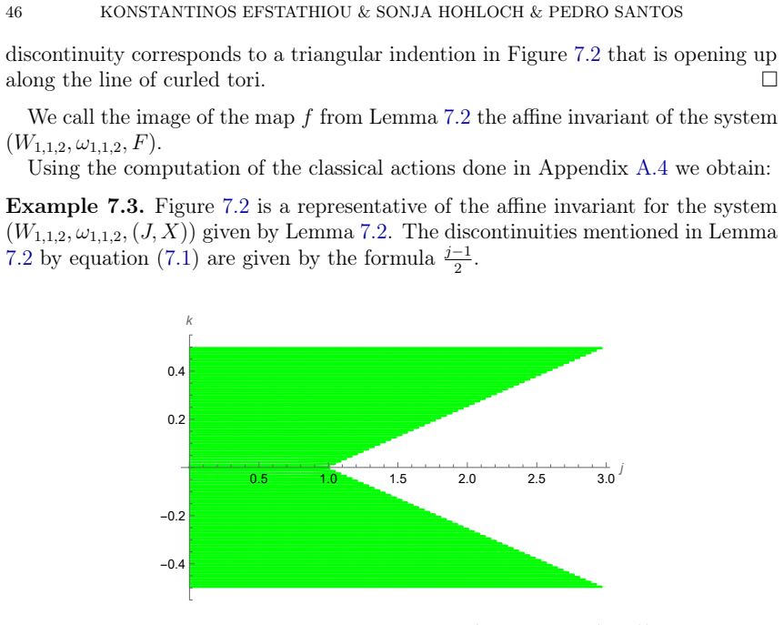
Figure 7.2. Figure 7.2: Classical actions of the system (W1,1,2, ω1,1,2,(J, X)) evalu￾ated on the joint spectrum for ℏ = 0.01. Remark 7.4. Analogously to Section 5.2 and Section 5.5 a vertical cut could be made at the value c(1), obtaining maps f1 and f2 in each connected component. The map f2 can be continuously extended to f1 by applying the transformation f2 − (J−1) 2 . Notice that this transformation is not affine. However,… view at source ↗
Figure 7.3
Figure 7.3. Figure 7.3: Bifurcation diagram for the system (W1,1,2, ω1,1,2,(J, H)) to￾gether with its joint spectrum for ℏ = 0.05. The bifurcation diagram is sketched in red. The degenerate, non parabolic value in the interior of F(M) is indicated in black. The values from the joint spectrum are plotted in blue. 0.80 0.85 0.90 0.95 1.00 1.05 1.10 1.15 1.20 j 0.66 0.68 0.70 0.72 0.74 0.76 0.78 h [PITH_FULL_IMAGE:figures/full_fi… view at source ↗
Figure 7.4
Figure 7.4. Figure 7.4: Bifurcation diagram of the system together with its joint spec￾trum, for ℏ = 0.01, in the range (j, h) ∈ [0.8, 1.2] × [0.65, 0.78]. The gen￾eralized flap can be seen to appear. The bifurcation diagram is sketched in black. The orange point represents the degenerate value. Green points correspond to values in the joint spectrum outside of the generalized flap. Red points correspond to values in the joint … view at source ↗
Figure 7.5
Figure 7.5. Figure 7.5: Classical actions of the system (W1,1,2, ω1,1,2,(J, H)) com￾puted on the joint spectrum for ℏ = 0.01. On the left the classical actions are computed in the background of the system. Green points correspond to values outside of the generalized flap. Red points correspond to values on the background of the generalized flap. On the right the classical actions are computed in the flappy part of the generaliz… view at source ↗
Figure 8.1
Figure 8.1. Figure 8.1: Bifurcation diagram for the system (W1,1,2, ω1,1,2, Fa,b,c) with (a, b, c) = (20, −35, 17) together with the joint spectrum for ℏ = 1 25 . The purple points correspond to focus-focus values. The black points correspond to hyperbolic-regular values. The orange points correspond to parabolic values. The brown points correspond to elliptic-regular values. The pink points correspond to elliptic-elliptic valu… view at source ↗
Figure 8.2
Figure 8.2. Figure 8.2: Bifurcation diagram for the system (W1,1,2, ω1,1,2, Fa,b,c) with (a, b, c) = ( √ 20 2 , −√ 35 2 , √ 17 2 ) together with the joint spectrum for ℏ = 1 25 . The purple points correspond to focus-focus values. The black points correspond to hyperbolic-regular values. The orange points correspond to parabolic values. The brown points correspond to elliptic-regular values. The pink points correspond to ellipt… view at source ↗
Figure 8.3
Figure 8.3. Figure 8.3: Bifurcation diagram for the system (W1,1,2, ω1,1,2, Fa,b,c) with (a, b, c) = (100, −200, 110) together with its joint spectrum for ℏ = 1 25 . The purple points correspond to elliptic-elliptic values. The black points correspond to hyperbolic-regular values. The orange points correspond to parabolic values. The brown points correspond to elliptic-regular values. The pink points correspond to elliptic-elli… view at source ↗
Figure 8.4
Figure 8.4. Figure 8.4: Representatives of the affine invariant given by Theorem 8.2 applied to the joint spectrum of the system (W1,1,2, ω1,1,2, Fa,b,c) with (a, b, c) = (20, −35, 17) and ℏ = 1 25 . The green points correspond to the classical actions computed outside of the flap. The red points correspond to the classical actions computed on the background of the flap. The blue points correspond to the classical actions compu… view at source ↗
Figure 8.5
Figure 8.5. Figure 8.5: Representatives of the affine invariant given by Theorem 8.2 applied to the joint spectrum of the system (W1,1,2, ω1,1,2, Fa,b,c) with (a, b, c) = ( √ 20 2 , − √ 35 2 , √ 17 2 ) and ℏ = 1 50 . The green points correspond to the classical actions computed outside of the flap. The red points correspond to the classical actions computed on the background of the flap. The blue points correspond to the classi… view at source ↗
Figure 8.6
Figure 8.6. Figure 8.6: Representatives of the affine invariant given by Theorem 8.2 applied to the joint spectrum of the system (W1,1,2, ω1,1,2, Fa,b,c) with (a, b, c) = (100, 200, −110) and ℏ = 1 25 . The green points correspond to the classical actions computed outside of the initial flap. The red points cor￾respond to the classical actions computed on the background of the initial flap. The blue points correspond to the cla… view at source ↗
read the original abstract

Hypersemitoric systems are a class of integrable systems on $4$-dimensional symplectic manifolds which only have mildly degenerate singularities and where one of the integrals induces an effective Hamiltonian $S^1$-action and is proper. We introduce the affine invariant of hypersemitoric systems, which is a generalization of the Delzant polytope of toric systems and the polytope invariant of semitoric systems. Along the way, we compute and plot this invariant for meaningful and more and more complicated examples.

Editorial analysis

A structured set of objections, weighed in public.

Desk editor's note, referee report, simulated authors' rebuttal, and a circularity audit. Tearing a paper down is the easy half of reading it; the pith above is the substance, this is the friction.

Referee Report

0 major / 2 minor

Summary. The manuscript defines hypersemitoric systems as 4-dimensional integrable systems possessing only mildly degenerate singularities with one integral inducing a proper effective Hamiltonian S¹-action. It introduces an affine invariant that generalizes the Delzant polytope of toric systems and the polytope invariant of semitoric systems, and computes and plots the invariant on a sequence of explicit examples of increasing complexity.

Significance. If rigorously established, the affine invariant would extend the polytope-based classification program to a larger class of 4D integrable systems. The explicit computations and plots on concrete examples constitute a concrete strength, allowing direct verification of the construction and its reduction to the toric and semitoric cases.

minor comments (2)
  1. A summary table listing the examples, their singularity data, and the computed affine invariants would improve readability and allow quick comparison across the sequence of examples.
  2. Figure captions and axis labels should explicitly reference the specific hypersemitoric system under consideration to avoid ambiguity when multiple plots appear in the same section.

Simulated Author's Rebuttal

0 responses · 0 unresolved

We thank the referee for their careful reading, positive summary of the manuscript, and recommendation for minor revision. No specific major comments were raised in the report.

Circularity Check

0 steps flagged

No significant circularity identified

full rationale

The manuscript defines the class of hypersemitoric systems from standard symplectic data (mildly degenerate singularities plus a proper effective Hamiltonian S¹-action) and constructs the affine invariant directly as a generalization of the Delzant and semitoric polytopes. No load-bearing step reduces by definition, fitted parameter, or self-citation chain to its own inputs; the central claim is an explicit construction demonstrated on examples. The derivation is therefore self-contained against external benchmarks.

Axiom & Free-Parameter Ledger

0 free parameters · 0 axioms · 0 invented entities

Abstract alone identifies no explicit free parameters, axioms, or invented entities; the construction appears to rest on standard definitions of integrable systems and S1-actions in the field.

pith-pipeline@v0.9.0 · 5612 in / 1011 out tokens · 37203 ms · 2026-05-23T17:31:29.058856+00:00 · methodology

discussion (0)

Sign in with ORCID, Apple, or X to comment. Anyone can read and Pith papers without signing in.

Reference graph

Works this paper leans on

7 extracted references · 7 canonical work pages

  1. [1]

    Normalisationofthesmoothfocus-focus:asimpleproof

    issn: 1364-503X,1471-2962. doi: 10.1098/rsta.2017.0424 . url: https://doi.org/10.1098/rsta.2017.0424. 66 REFERENCES [Can01] Ana Cannas da Silva. Lectures on symplectic geometry. Vol. 1764. Lecture Notes in Mathematics. Springer-Verlag, Berlin, 2001, pp. xii+217.isbn: 3-540-42195-5. doi: 10.1007/978-3-540-45330-7 . url: https://doi. org/10.1007/978-3-540-4...

  2. [2]

    doi: 10.1016/j.geomphys.2016.05

    issn: 0393-0440,1879-1662. doi: 10.1016/j.geomphys.2016.05

  3. [3]

    Integrable Hamiltonian systems with swal- lowtails

    url: https://doi.org/10.1016/j.geomphys.2016.05.014. [ES10] K. Efstathiou and D. Sugny. “Integrable Hamiltonian systems with swal- lowtails”.In:J. Phys. A43.8(2010),pp.085216,25. issn:1751-8113,1751-

  4. [4]

    Convexitypropertiesofthemomentmap- ping

    doi: 10.1088/1751-8113/43/8/085216. url: https://doi.org/ 10.1088/1751-8113/43/8/085216. [GS82] V.GuilleminandS.Sternberg.“Convexitypropertiesofthemomentmap- ping”. In:Invent. Math.67.3 (1982), pp. 491–513.issn: 0020-9910,1432-

  5. [5]

    Extending compact Hamiltonian S1- spaces to integrable systems with mild degeneracies in dimension four

    doi: 10.1007/BF01398933 . url: https://doi.org/10.1007/ BF01398933. [HP21] Sonja Hohloch and Joseph Palmer. “Extending compact Hamiltonian S1- spaces to integrable systems with mild degeneracies in dimension four”. In: arxiv prepint arXiv:2105.00523 (2021). url: https://arxiv.org/ abs/2105.00523. [Kar99] Yael Karshon. “Periodic Hamiltonian flows on four-d...

  6. [6]

    Über das Verhalten analytischer Hamiltonscher Dif- ferentialgleichungen in der Nähe einer Gleichgewichtslösung

    issn: 0010-3616,1432-0916. doi: 10 . 1007 / s00220 - 011 - 1360 - 4. url: https://doi.org/10.1007/s00220-011-1360-4. [Rüs64] Helmut Rüssmann. “Über das Verhalten analytischer Hamiltonscher Dif- ferentialgleichungen in der Nähe einer Gleichgewichtslösung”. In:Math. Ann. 154 (1964), pp. 285–300.issn: 0025-5831,1432-1807.doi: 10.1007/ BF01362565. url: https:...

  7. [7]

    Smooth normal forms for in- tegrable Hamiltonian systems near a focus-focus singularity

    doi: 10.1016/j.aim.2006.04.004 . url: https://doi.org/10. 1016/j.aim.2006.04.004. [VW13] San Vu Ngoc and Christophe Wacheux. “Smooth normal forms for in- tegrable Hamiltonian systems near a focus-focus singularity”. In:Acta Math. Vietnam. 38.1 (2013), pp. 107–122.issn: 0251-4184,2315-4144. doi: 10 . 1007 / s40306 - 013 - 0012 - 5. url: https : / / doi . o...