REVIEW 4 major objections 8 minor 50 references
A Semi-Lagrangian Adaptive-Rank (SLAR) Method for Linear Advection and Nonlinear Vlasov-Poisson System
T0 review · 4 major / 8 minor · reviewed 2026-08-12 · deepseek-v4-flash
Pith's one-line read The SLAR method updates only sampled rows and columns of the phase-space solution, achieving a high-order, locally conservative semi-Lagrangian kinetic solver whose cost grows linearly with mesh size.
desk verdict Promising non-splitting low-rank semi-Lagrangian scheme for linear advection; the Vlasov-Poisson extension has an unclosed LoMaC correction step that undercuts the headline complexity and conservation claims. read the letter →
The pith
A machine-rendered reading of the paper's core claim, the machinery that carries it, and where it could break.
The reading
What carries the argument
The engine is adaptive cross approximation (CUR, or pseudo-skeleton decomposition) of the solution matrix, in which representative columns and rows are picked greedily from the entries with largest residual and combined through a recursive rank-one update. This builds $A\approx E_JDE_I$ without forming the full matrix, and in SLAR the entries it asks for are supplied on demand by a compact third-order semi-Lagrangian finite-difference reconstruction at the feet of backward characteristics. A wider SVD truncation threshold than the cross tolerance is then applied, so spurious high-frequency modes introduced by interpolation are filtered out and the rank stays small. For the nonlinear Vlasov-Poisson system the same machinery runs inside a Runge-Kutta exponential integrator that freezes the electric field at each stage, while an implicit upwind discretization of the charge-density equation plus a LoMaC Maxwellian correction enforces local mass conservation without reducing the allowed time step.
What would settle it
Take a two-dimensional linear advection initial condition whose exact solution has slowly decaying singular values (for example, a sum of sharp Gaussian blobs arranged so the singular-value spectrum stays above $\epsilon_C$ for hundreds of modes). Run SLAR on a $256 \times 256$ grid and compare the recovered rank and the $L^1$ error against a full-rank reference at one time step. If the cross approximation needs more than a small constant number $r$ of rows and columns, or the SVD-truncated solution deviates by more than $\epsilon_S$, the $O(Nr)$ complexity and accuracy claims are falsified.
Extended reading notes
Core claim
The central claim is that a non-splitting semi-Lagrangian finite-difference solver can be fused with adaptive cross approximation to produce the first adaptive-rank semi-Lagrangian method that is high order, stable at large time steps, and locally mass-conserving. On a two-dimensional tensor-product grid the solution is kept as an SVD $F^n = U^n\Sigma^n(V^n)^\top$; at each step a greedy pivot search selects representative rows and columns, the local semi-Lagrangian solver evaluates only those entries by tracing characteristics to their feet, and a recursive cross update builds the factorization $\tilde F^{n+1}=E_JD E_I$. An SVD truncation with a threshold larger than the cross tolerance then removes numerical noise and keeps the rank low. For Vlasov-Poisson, characteristics are tracked with a third-order Runge-Kutta exponential integrator, and local charge conservation is restored by solving the macroscopic density equation implicitly and applying a LoMaC correction that reshapes the distribution with a local Maxwellian. The benchmark results report third-order convergence, adaptive rank behavior, compression ratios that improve as the mesh is refined, and matching decay and growth rates for Landau damping.
Load-bearing premise
The whole efficiency argument depends on the solution matrix having a rapidly decaying singular-value spectrum at every time step, and on the greedy random sampling of rows and columns finding that low-rank structure reliably; when either fails, the rank and the cost grow.
Editorial extensions
If this is right
- Per time step, the cost is $O(Nr + r^3)$ per dimension after accounting for the local SL evolutions, the SVD truncation, and the implicit density solve, so refined meshes cost linearly rather than quadratically.
- Time steps set by CFL numbers as large as 100 still show third-order temporal accuracy, so the method converts spatial resolution into accuracy without being throttled by the fastest wave in the system.
- Local conservation of charge density holds at large time steps because the density is updated implicitly and then enforced through a LoMaC correction, removing the extra stability constraint identified in earlier conservative SL-FD schemes.
- The SVD truncation with $\epsilon_S > \epsilon_C$ removes modes generated by numerical error, which keeps the recorded rank near the intrinsic rank of the solution even when the cross approximation oversamples.
- For the nonlinear Vlasov-Poisson benchmarks, the method reproduces the standard Landau damping rates and bump-on-tail growth with ranks far below the grid dimension.
Reading between the lines
- The on-demand evaluation structure means the same CUR-plus-truncation skeleton could be attached to other high-order spatial reconstructions or lifted to tensor-train formats; the paper only demonstrates the 2D matrix case and names higher dimensions as future work.
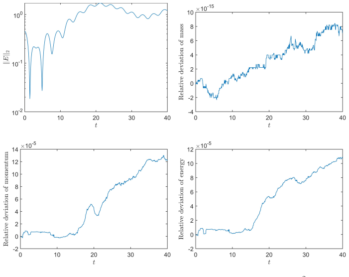
- Because the LoMaC correction enforces only the zeroth moment, momentum and energy conservation are reported as residual deviations at the tolerance level; a natural extension would preserve additional moments, which the paper does not address.
- The pivot search starts from random samples, so different runs may select different rows and columns; an untested but easy stress test is to repeat the benchmarks over many random seeds and compare error and rank distributions.
- If long-time Vlasov filamentation causes singular values to decay slowly, the rank will grow and the $O(Nr)$ advantage will erode; the demonstrated complexity advantage is therefore for the finite-time benchmark window, not a proven long-time guarantee.
Editorial analysis
A structured set of objections, weighed in public.
Referee Report
Summary. This paper proposes a semi-Lagrangian adaptive-rank (SLAR) method for linear advection equations and for the 1D1V Vlasov-Poisson system. The method combines a local non-splitting finite-difference semi-Lagrangian update with adaptive cross approximation (CUR) for the 'step' phase and SVD truncation for the 'truncate' phase. For the VP system, the authors use a Runge-Kutta exponential integrator for characteristic tracing, an implicit upwind/DIRK solver for the macroscopic charge-density equation, and a LoMaC-type Maxwellian correction to enforce local charge conservation. The central claims are third-order accuracy in space and time, large-time-step stability, adaptivity of rank, local charge conservation, and O(N r) complexity per time step. Numerical benchmarks include linear advection with constant coefficients, rigid-body rotation, swirling deformation flow, weak/strong Landau damping, and bump-on-tail instability, with convergence tables, rank histories, conservation diagnostics, damping-rate measurements, and a complexity scaling plot.
Significance. If the algorithm is made precise and the claims are verified, the contribution is significant: it appears to be the first non-splitting high-order adaptive-rank semi-Lagrangian method for kinetic equations, and the combination of ACA sampling with SL-FD updates is novel. The paper ships extensive numerical evidence: convergence orders in Table 3.1 and Figures 3.4 and 3.11, rank histories in Figures 3.6, 3.9, 3.12, and 3.14, conservation diagnostics in Figures 3.10 and 3.15, damping rates matching theory in Figure 3.8, and a linear-complexity scaling plot in Figure 3.13. These tests go well beyond a single toy problem. However, the manuscript is a numerical-methods paper without error or stability analysis, and two central algorithmic specifications--the SVD rank-selection rule and the use of the LoMaC-corrected solution in the next time step--are not correct or complete as written. Those issues must be resolved before the main claims can be accepted.
major comments (4)
- [Algorithm 3, line 4] The rank-selection rule `r_S <- min{k | (Sigma_S)_{k+1,k+1} > epsilon_S}` is not a valid truncation rule. As written, it returns the first index whose trailing singular value exceeds the tolerance, and for k = r_C it refers to the out-of-range index r_C + 1. If the first few singular values are above epsilon_S, the rule either returns 1 when more modes should be kept or returns no valid index and performs no truncation. The intended rule is almost certainly `r_S <- max{k | (Sigma_S)_{k,k} > epsilon_S}` or equivalently `min{k | (Sigma_S)_{k+1,k+1} <= epsilon_S}`. Since the SVD truncation is the stability and complexity control of the whole SLAR method, this is a load-bearing specification error, not a typographical nicety.
- [Section 2.2.2, Eq. (2.25)] The nonlinear time-stepping loop is not closed. Algorithm 3 and Eq. (2.14) require the input F^n to be a low-rank SVD matrix U Sigma V^T, and the next RK stage or next time step is invoked on the output of the scheme. However, after the LoMaC correction (2.25), F^{n+1} = F^{n+1,*} + M^{n+1} - M^{n+1,*}, and the paper explicitly states that this is 'no necessarily in the low rank format.' No recompression, projection, or factored representation of the corrected sum is specified. If one truncates F^{n+1} to restore the input format, the truncation changes the matrix entries and hence the local charge densities that (2.25) was designed to conserve, and no conservation or error bound is provided. If one does not truncate, the next invocation of Algorithm 1/3 receives a representation not covered by the algorithm's stated input, and the claimed O(N r) storage and complexity accounting does not apply to the full correction term. If the intended implementation carries the correction in a special structured form and evaluates entries on the fly, that representation must be stated and analyzed. The conservation diagnostics in Figures 3.10 and 3.15 test only the corrected solution at the end of a step and do not expose this issue.
- [Abstract and Section 2.1.3 / Algorithm 3] The abstract claims that the method applies 'singular value truncation and a mass-conservative projection following the cross approximation of the updated solution,' but for the linear-advection SLAR method in Algorithm 3 there is no mass-conservative projection after the SVD truncation; the only correction step is the LoMaC Maxwellian correction introduced later for the nonlinear VP system. If the mass-conservation claim is intended only for the VP system, this should be stated explicitly; if it is intended for the linear SLAR method as well, the missing projection must be specified, because SVD truncation does not preserve local or even global mass in general.
- [Section 2.1.2, Algorithm 1] The ACA pivot selection is a random sampling plus greedy search heuristic, and the stopping criterion in line 8 bounds only the norm of the rank-one update, not the distance between the cross approximation and the exact updated solution. The paper provides no error estimate or failure diagnostic for this selection, and no sensitivity study with respect to the number p of random samples. Since the accuracy and the O(N r) complexity claims rest on the assumption that the sampled rows and columns capture the dominant low-rank modes of the solution at every step, this missing control is a substantive gap; at minimum the authors should state the working assumptions and report the sensitivity of the results to p and to the random seed.
minor comments (8)
- [Algorithm 1, line 5] The second greedy search should use a new row index j_k^*, not i_k^*; as typeset, both lines 4 and 5 write i_k^*.
- [Eqs. (2.7)-(2.9)] The definition of the reconstruction operator R as a minimum of a least-squares residual is inconsistent with its use as the interpolated polynomial value; the coefficients in (2.9) should be presented directly as the reconstruction, and the optimization description should be corrected, for example by writing p = argmin and R = p(x,y).
- [Eq. (3.1)] The time-step formula is typeset ambiguously; it should read Delta t = CFL / (max{|a|}/Delta x + max{|b|}/Delta y).
- [Abstract and Section 2.2.1] The text contains typos: 'The propose algorithm' and 'expontential integrators' should be corrected to 'The proposed algorithm' and 'exponential integrators'.
- [Figure 3.8 caption] The caption says 'electric filed'; it should say 'electric field'.
- [Algorithms 1 and 2] The number p of random samples in Algorithm 1 and the number s of sample points per edge in Algorithm 2 are never specified; stating default values and, ideally, reporting variance over random seeds would materially improve reproducibility.
- [Section 3.2, Figure 3.10] The conservation test uses the velocity domain [-10,10] while other strong-Landau runs use [-2 pi, 2 pi]; this difference should be stated in the caption or text to avoid confusion.
- [Section 2.1.3] The statement that the SVD truncation is 'closely related to that of [2]' is vague; a precise statement of which oversampling property or error bound is being invoked would be helpful.
Circularity Check
No significant circularity: SLAR is a constructive algorithm whose claimed conservation and accuracy are validated against external benchmarks; the nonlinear low-rank closure gap is a correctness concern, not circularity.
full rationale
I examined the claimed derivation chain. The SLAR method is assembled from explicit algorithmic components: the local SL-FD reconstruction (Eqs. (2.6)-(2.10)), the ACA/CUR approximation (Algorithm 1 with Proposition 2.1), SVD truncation (Algorithm 3), the RK exponential integrator (Eqs. (2.17)-(2.18)), and the LoMaC correction (Eq. (2.25)). No parameter is fitted to benchmark data and then presented as a prediction, and no quantity is defined in terms of the quantity it is claimed to predict. The low-rank representation (2.2) is stated as an assumption, not derived from the target accuracy or conservation results. The LoMaC correction enforces local charge conservation by construction: after Eq. (2.25), the zeroth moment of F^{n+1} equals rho^{n+1} because M^{n+1} and M^{n+1,*} differ only in the density factor. The paper does not present this as an independent first-principles discovery, so this is a design guarantee, not circularity. The self-citations [4, 29, 30, 45, 49] supply published building blocks (RK exponential integrators, LoMaC correction, recursive cross updates, conservative SL-FD methods) rather than restating the target result. The central novelty claim is tested against exact solutions (Example 3.1), known Landau damping rates, and a dense-mesh reference SL-FV solver [50], providing independent validation. A genuine non-circularity concern is present: the paper states that after the LoMaC correction the solution is 'a summation of low rank prediction and an explicit correction term in Maxwellian form (no necessarily in the low rank format)' (Section 2.2.2), and no subsequent truncation or projection is specified before the next SLAR call. This creates an algorithmic closure and complexity risk, since the next iteration expects a low-rank SVD input and the O(Nr) complexity accounting omits the cost of the full correction term. However, this is a correctness/completeness issue, not a reduction of the claimed result to its own inputs, so it does not constitute circularity.
Assumptions & free parameters
free parameters (5)
- epsilon_C (cross approximation tolerance) =
10^-4 (default), 10^-5 (weak Landau damping)
- epsilon_S (SVD truncation tolerance) =
10^-3 (default), 10^-4 (weak Landau damping)
- p (random samples per ACA iteration) =
not specified
- Index range expansion (+/- 2 cells) =
2
- CFL number =
1 or 10 (tests), up to 100 (accuracy study)
assumptions (6)
- domain assumption The numerical solution on the tensor-product grid admits a low-rank SVD representation with rapidly decaying singular values at every time step.
- domain assumption The greedy cross approximation with random seeding (Algorithm 1) finds a near-optimal set of rows and columns with controllable error.
- standard math The third-order local least-squares reconstruction in Eq. (2.8) is accurate and stable on the unsplit SL-FD stencil.
- standard math The RK exponential integrator with frozen velocity fields (Butcher table (2.17)) accurately traces nonlinear characteristics for the VP system to third order.
- ad hoc to paper The LoMaC correction localizes the density error with a local Maxwellian (Eq. (2.25)), and the resulting F^{n+1} is an adequate phase-space distribution.
- ad hoc to paper The boundary tracing in Algorithm 2 correctly predicts the support of the advected solution.
Cite this review
Pith. "Pith review of A Semi-Lagrangian Adaptive-Rank (SLAR) Method for Linear Advection and Nonlinear Vlasov-Poisson System." pith.science (2026). https://pith.science/paper/VTSB2OOI
@misc{pith2026241117963,
  author       = {Pith},
  title        = {Pith review of: A Semi-Lagrangian Adaptive-Rank (SLAR) Method for Linear Advection and Nonlinear Vlasov-Poisson System},
  year         = {2026},
  howpublished = {\url{https://pith.science/paper/VTSB2OOI}},
  note         = {Machine review of arXiv:2411.17963}
}
abstract
High-order semi-Lagrangian methods for kinetic equations have been under rapid development in the past few decades. In this work, we propose a semi-Lagrangian adaptive rank (SLAR) integrator in the finite difference framework for linear advection and nonlinear Vlasov-Poisson systems without dimensional splitting. The proposed method leverages the semi-Lagrangian approach to allow for significantly larger time steps while also exploiting the low-rank structure of the solution. This is achieved through cross approximation of matrices, also referred to as CUR or pseudo-skeleton approximation, where representative columns and rows are selected using specific strategies. To maintain numerical stability and ensure local mass conservation, we apply singular value truncation and a mass-conservative projection following the cross approximation of the updated solution. The computational complexity of our method scales linearly with the mesh size $N$ per dimension, compared to the $\mathcal{O}(N^2)$ complexity of traditional full-rank methods per time step. The algorithm is extended to handle nonlinear Vlasov-Poisson systems using a Runge-Kutta exponential integrator. Moreover, we evolve the macroscopic conservation laws for charge densities implicitly, enabling the use of large time steps that align with the semi-Lagrangian solver. We also perform a mass-conservative correction to ensure that the adaptive rank solution preserves macroscopic charge density conservation. To validate the efficiency and effectiveness of our method, we conduct a series of benchmark tests on both linear advection and nonlinear Vlasov-Poisson systems. The propose algorithm will have the potential in overcoming the curse of dimensionality for beyond 2D high dimensional problems, which is the subject of our future work.
Figures


Figures from the paper (12 more)


Reference graph
Works this paper leans on
-
[1]
R. Alexander, Diagonally implicit Runge–Kutta methods for stiff ODE’s , SIAM Journal on Numerical Analysis, 14 (1977), pp. 1006–1021. 21
work page 1977
-
[2]
D. Anderson, S. Du, M. Mahoney, C. Melgaard, K. Wu, and M. Gu , Spectral gap error bounds for improving cur matrix decomposition and the nystr¨ om method , in Artificial intelligence and statistics, PMLR, 2015, pp. 19–27
work page 2015
-
[3]
Bebendorf , Approximation of boundary element matrices , Numerische Mathematik, 86 (2000), pp
M. Bebendorf , Approximation of boundary element matrices , Numerische Mathematik, 86 (2000), pp. 565–589
2000
-
[4]
X. Cai, S. Boscarino, and J.-M. Qiu , High order semi-lagrangian discontinuous galerkin method coupled with runge-kutta exponential integrators for nonlinear vlasov dynamics, Journal of Computational Physics, 427 (2021), p. 110036
work page 2021
-
[5]
X. Cai, W. Guo, and J.-M. Qiu , A high order semi-Lagrangian discontinuous Galerkin method for Vlasov–Poisson simulations without operator splitting , Journal of Computational Physics, 354 (2018), pp. 529–551
work page 2018
-
[6]
J. Carpio and J. Prieto , An anisotropic, fully adaptive algorithm for the solution of convection-dominated equations with semi-Lagrangian schemes, Computer Methods in Applied Mechanics and Engineering, 273 (2014), pp. 77–99
work page 2014
-
[7]
J. A. Carrillo and F. Vecil , Nonoscillatory interpolation methods applied to Vlasov-based models, SIAM Journal on Scientific Computing, 29 (2007), pp. 1179–1206
work page 2007
-
[8]
Ceruti and C
G. Ceruti and C. Lubich , An unconventional robust integrator for dynamical low-rank approximation, BIT Numerical Mathematics, 62 (2022), pp. 23–44
2022
Show all 50 references
-
[9]
Chaturantabut and D
S. Chaturantabut and D. C. Sorensen, Nonlinear model reduction via discrete empirical interpolation, SIAM Journal on Scientific Computing, 32 (2010), pp. 2737–2764
2010
-
[10]
Cheng and G
C.-Z. Cheng and G. Knorr , The integration of the Vlasov equation in configuration space , Journal of Computational Physics, 22 (1976), pp. 330–351
1976
-
[11]
Civril and M
A. Civril and M. Magdon-Ismail , Finding maximum volume sub-matrices of a matrix , RPI Comp Sci Dept TR, (2007), pp. 07–08
2007
-
[12]
Cortinovis and L
A. Cortinovis and L. Ying, A sublinear-time randomized algorithm for column and row sub- set selection based on strong rank-revealing qr factorizations, arXiv preprint arXiv:2402.13975, (2024)
2024 arXiv
-
[13]
Cristiani and M
E. Cristiani and M. F alcone, Fast semi-Lagrangian schemes for the Eikonal equation and applications, SIAM Journal on Numerical Analysis, 45 (2007), pp. 1979–2011
2007
-
[14]
Dektor , A collocation method for nonlinear tensor differential equations on low-rank manifolds, arXiv preprint arXiv:2402.18721, (2024)
A. Dektor , A collocation method for nonlinear tensor differential equations on low-rank manifolds, arXiv preprint arXiv:2402.18721, (2024)
2024 arXiv
-
[15]
Dektor, A
A. Dektor, A. Rodgers, and D. Venturi , Rank-adaptive tensor methods for high- dimensional nonlinear pdes , Journal of Scientific Computing, 88 (2021), p. 36
2021
-
[16]
Dolgov and D
S. Dolgov and D. Savostyanov, Parallel cross interpolation for high-precision calculation of high-dimensional integrals , Computer Physics Communications, 246 (2020), p. 106869
2020
-
[17]
Drineas, M
P. Drineas, M. W. Mahoney, and S. Muthukrishnan , Relative-error cur matrix decom- positions, SIAM Journal on Matrix Analysis and Applications, 30 (2008), pp. 844–881. 22
2008
-
[18]
Einkemmer and C
L. Einkemmer and C. Lubich , A low-rank projector-splitting integrator for the Vlasov– Poisson equation, SIAM Journal on Scientific Computing, 40 (2018), pp. B1330–B1360
2018
-
[19]
Einkemmer, A
L. Einkemmer, A. Ostermann, and C. Piazzola , A low-rank projector-splitting integra- tor for the Vlasov–Maxwell equations with divergence correction , Journal of Computational Physics, 403 (2020), p. 109063
2020
-
[20]
H. C. Elman , Iterative methods for large, sparse, nonsymmetric systems of linear equations , Yale University, 1982
1982
-
[21]
Engquist and L
B. Engquist and L. Ying , Fast directional multilevel algorithms for oscillatory kernels , SIAM Journal on Scientific Computing, 29 (2007), pp. 1710–1737
2007
-
[22]
Filbet, E
F. Filbet, E. Sonnendr ¨ucker, and P. Bertrand , Conservative numerical schemes for the Vlasov equation , Journal of Computational Physics, 172 (2001), pp. 166–187
2001
-
[23]
Ghahremani and H
B. Ghahremani and H. Babaee , Cross interpolation for solving high-dimensional dynam- ical systems on low-rank tucker and tensor train manifolds , Computer Methods in Applied Mechanics and Engineering, 432 (2024), p. 117385
2024
-
[24]
S. A. Goreinov, E. E. Tyrtyshnikov, and N. L. Zamarashkin, A theory of pseudoskele- ton approximations, Linear algebra and its applications, 261 (1997), pp. 1–21
1997
-
[25]
Grasedyck, Hierarchical singular value decomposition of tensors, SIAM journal on matrix analysis and applications, 31 (2010), pp
L. Grasedyck, Hierarchical singular value decomposition of tensors, SIAM journal on matrix analysis and applications, 31 (2010), pp. 2029–2054
2010
-
[26]
Grasedyck, R
L. Grasedyck, R. Kriemann, C. L ¨obbert, A. N¨agel, G. Wittum, and K. Xylouris , Parallel tensor sampling in the hierarchical tucker format , Computing and visualization in science, 17 (2015), pp. 67–78
2015
-
[27]
W. Guo, J. F. Ema, and J.-M. Qiu , A Local Macroscopic Conservative (LoMaC) low rank tensor method with the discontinuous Galerkin method for the Vlasov dynamics , Communica- tions on Applied Mathematics and Computation, 6 (2024), pp. 550–575
2024
-
[28]
Guo and J.-M
W. Guo and J.-M. Qiu , A low rank tensor representation of linear transport and nonlinear Vlasov solutions and their associated flow maps, Journal of Computational Physics, 458 (2022), p. 111089
2022
-
[29]
Guo and J.-M
W. Guo and J.-M. Qiu , A conservative low rank tensor method for the Vlasov dynamics , SIAM Journal on Scientific Computing, 46 (2024), pp. A232–A263
2024
-
[30]
, A local macroscopic conservative (lomac) low rank tensor method for the vlasov dynam- ics, Journal of Scientific Computing, (to appear)
-
[31]
Koch and C
O. Koch and C. Lubich , Dynamical low-rank approximation , SIAM Journal on Matrix Analysis and Applications, 29 (2007), pp. 434–454
2007
-
[32]
Kormann , A semi-Lagrangian Vlasov solver in tensor train format , SIAM Journal on Scientific Computing, 37 (2015), pp
K. Kormann , A semi-Lagrangian Vlasov solver in tensor train format , SIAM Journal on Scientific Computing, 37 (2015), pp. B613–B632
2015
-
[33]
Kressner and C
D. Kressner and C. Tobler , Algorithm 941: Htucker—a matlab toolbox for tensors in hierarchical tucker format, ACM Transactions on Mathematical Software (TOMS), 40 (2014), pp. 1–22. 23
2014
-
[34]
P. H. Lauritzen, R. D. Nair, and P. A. Ullrich , A conservative semi-Lagrangian multi- tracer transport scheme (CSLAM) on the cubed-sphere grid, Journal of Computational Physics, 229 (2010), pp. 1401–1424
2010
-
[35]
M. W. Mahoney and P. Drineas , Cur matrix decompositions for improved data analysis , Proceedings of the National Academy of Sciences, 106 (2009), pp. 697–702
2009
-
[36]
I. V. Oseledets , Tensor-train decomposition, SIAM Journal on Scientific Computing, 33 (2011), pp. 2295–2317
2011
-
[37]
T. N. Phillips and A. J. Williams, A semi-Lagrangian finite volume method for Newtonian contraction flows, SIAM Journal on Scientific Computing, 22 (2001), pp. 2152–2177
2001
-
[38]
Puigferrat, M
A. Puigferrat, M. Mas´o, I. De-Pouplana, G. Casas, and E. O˜nate, Semi-Lagrangian formulation for the advection–diffusion–absorption equation , Computer methods in applied mechanics and engineering, 380 (2021), p. 113807
2021
-
[39]
Qiu and C.-W
J.-M. Qiu and C.-W. Shu , Positivity preserving semi-Lagrangian discontinuous Galerkin formulation: theoretical analysis and application to the Vlasov–poisson system , Journal of Computational Physics, 230 (2011), pp. 8386–8409
2011
-
[40]
Restelli, L
M. Restelli, L. Bonaventura, and R. Sacco, A semi-Lagrangian discontinuous Galerkin method for scalar advection by incompressible flows , Journal of Computational Physics, 216 (2006), pp. 195–215
2006
-
[41]
J. A. Rossmanith and D. C. Seal , A positivity-preserving high-order semi-Lagrangian discontinuous Galerkin scheme for the Vlasov–Poisson equations , Journal of Computational Physics, 230 (2011), pp. 6203–6232
2011
-
[42]
T. F. Russell and M. A. Celia , An overview of research on Eulerian–Lagrangian localized adjoint methods (ELLAM) , Advances in Water resources, 25 (2002), pp. 1215–1231
2002
-
[43]
Saad and M
Y. Saad and M. H. Schultz, GMRES: A generalized minimal residual algorithm for solving nonsymmetric linear systems , SIAM Journal on scientific and statistical computing, 7 (1986), pp. 856–869
1986
-
[44]
W. A. Sands, W. Guo, J.-M. Qiu, and T. Xiong, High-order adaptive rank integrators for multi-scale linear kinetic transport equations in the hierarchical tucker format , arXiv preprint arXiv:2406.19479, (2024)
2024 arXiv
-
[45]
T. Shi, D. Hayes, and J.-M. Qiu , Distributed memory parallel adaptive tensor-train cross approximation, arXiv preprint arXiv:2407.11290, (2024)
2024 arXiv
-
[46]
D. C. Sorensen and M. Embree , A deim induced cur factorization , SIAM Journal on Scientific Computing, 38 (2016), pp. A1454–A1482
2016
-
[47]
G. W. Stewart , Four algorithms for the the efficient computation of truncated pivoted qr approximations to a sparse matrix , Numerische Mathematik, 83 (1999), pp. 313–323
1999
-
[48]
Tyrtyshnikov, S
E. Tyrtyshnikov, S. Goreinov, and N. Zamarashkin , Pseudo-skeleton approximations, Doklay Akdemii Nauk, 343 (1995), pp. 151–152. 24
1995
-
[49]
Xiong, G
T. Xiong, G. Russo, and J.-M. Qiu, Conservative multi-dimensional semi-Lagrangian finite difference scheme: stability and applications to the kinetic and fluid simulations , Journal of scientific computing, 79 (2019), pp. 1241–1270
2019
-
[50]
Zheng, X
N. Zheng, X. Cai, J.-M. Qiu, and J. Qiu , A fourth-order conservative semi-Lagrangian finite volume WENO scheme without operator splitting for kinetic and fluid simulations , Com- puter Methods in Applied Mechanics and Engineering, 395 (2022), p. 114973. 25
2022
Reviewed August 12, 2026 · model on record in the stance chip above.
Discussion (0). Continue with ORCID to comment.