A new method for studying the blazar variability on the shortest time scales and its application to S5 1803+784

A. S. Krivenko; M. A. Gorbachev; M. S. Butuzova; S. V. Nazarov; V. A. Guseva

REVIEW 4 major objections 5 minor 30 references

A new method for studying the blazar variability on the shortest time scales and its application to S5 1803+784

T0 review · 4 major / 5 minor · reviewed 2026-08-12 · deepseek-v4-flash

Challenge this review Re-run · record.json Download PDF Read on arXiv ↗ Review JSON

Pith's one-line read The paper proposes a sliding-window structure-function method and argues that S5 1803+784's hours-to-days optical flickering comes from jet sub-components with different volumes and Doppler factors.

desk verdict The new segment-by-segment structure-function method is worth reading, but the central Doppler-factor interpretation needs a red-noise null simulation before I'd believe it. read the letter →

arxiv 2411.18125 v1 pith:IUHRGVPW submitted 2024-11-27 astro-ph.HE

M. S. Butuzova , V. A. Guseva , M. A. Gorbachev , A. S. Krivenko , S. V. Nazarov This is my paper · ORCID

classification astro-ph.HE PACS 95.75.De95.75.Pq95.75.Wx98.54.Cm

keywords blazarvariabilityS51803+784structurefunctionTESSlightcurvescharacteristictimescaleDopplerfactoropticalphotometry

verification ladder T0 review T1 audit T2 compute T3 formal

The pith

A machine-rendered reading of the paper's core claim, the machinery that carries it, and where it could break.

The reading

This paper tries to establish that the rapid optical variability of the blazar S5 1803+784 is not a superposition of independent processes but the work of one continuous mechanism: a succession of sub-components in the jet, each with its own volume and Doppler factor, boosting the light on timescales from roughly half a day to five days. To see this, the authors introduce a method that slides along a continuous light curve, isolating consecutive intervals and measuring a characteristic variability time $\tau_v$ from the maximum of the structure function. Applied to TESS observations and cross-checked with multiband photometry, the method yields a correlation between variability amplitude and $\tau_v$ and no correlation between either quantity and the spectral index. A sympathetic reader would care because the result offers a single, geometrically motivated explanation for short-timescale blazar variability, and because the method is portable to other long, uniformly sampled datasets such as gamma-ray light curves.

What carries the argument

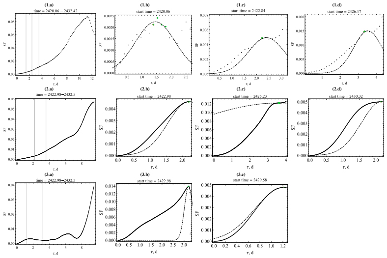
The machinery is a sliding-window structure-function analysis. The structure function $\mathrm{SF}(\tau)$ measures the mean squared flux difference between measurements separated by a lag $\tau$, and its maximum defines the characteristic variability time $\tau_v$. The method starts with the first twenty points of a continuous light curve, extends the window point by point until a structure-function maximum is found using slope-sign and amplitude thresholds, fits a Gaussian to the peak to refine $\tau_v$ and $\mathrm{SF}_{\max}$, discards that interval, and repeats along the whole series. The central assumption is that one variability process dominates at any given time, so each window carries a single $\tau_v$; significance is assessed by fitting ARIMA or ARMA models, generating 1000 simulated light curves, and counting how often their structure-function peaks reach the observed value.

What would settle it

Take a synthetic light curve built by adding two independently generated variability processes with known, different characteristic times, sample it at TESS cadence with comparable noise, and apply the proposed sliding-window method; if the recovered intervals systematically show a single $\tau_v$ with artificial jumps rather than the two injected timescales, the central claim loses its foundation. A second check is to examine one of the observed jumps in $\tau_v$ and see whether the spectral index from simultaneous multiband data changes discontinuously at that boundary, as the Doppler-subcomponent explanation requires.

Watch

Extended reading notes

Core claim

The central discovery claimed is that the shortest-timescale optical variability of S5 1803+784 is produced by the continuous appearance and evolution of sub-components of the emitting region with different volumes and Doppler factors $\delta = [\Gamma(1-\beta\cos\theta)]^{-1}$. In the observed TESS sector, the variability amplitude, measured by the structure-function maximum $\mathrm{SF}_{\max}$, grows with the characteristic time $\tau_v$, while the spectral index $\alpha$ correlates with neither. If Doppler-factor changes alone drove the variability, sub-components of equal volume would show a flatter spectrum and a shorter characteristic time at higher amplitude; the absence of a spectral-index correlation indicates that the sub-components differ in volume as well. The paper presents this as explaining both the amplitude-timescale correlation and the spectral independence within a single mechanism.

Load-bearing premise

The load-bearing premise is that at any moment one variability process dominates enough to define a single characteristic time; if several processes are active simultaneously, the sliding-window method will still output one timescale per window and can create segment boundaries that are artifacts of the assumption.

Editorial extensions

If this is right

The characteristic variability time of S5 1803+784 changes from roughly 0.5 to 5 days between adjacent intervals, sometimes by almost a factor of four, without a corresponding dependence on the object's brightness.
The positive correlation between $\mathrm{SF}_{\max}$ and $\tau_v$, strongest in aperture photometry with a Pearson coefficient near 0.97, implies that higher-amplitude fluctuations tend to last longer.
The lack of a correlation between spectral index and either $\mathrm{SF}_{\max}$ or $\tau_v$ implies that the emitting sub-components differ in volume, not only in Doppler factor.
The proposed method can be applied to other long, evenly sampled data series, such as gamma-ray monitoring of blazars, provided that gaps and noise are handled with explicit significance testing.

Reading between the lines

Editorial extensions of the paper, not claims the author makes directly.

I infer that the method's one-process-per-interval premise could be tested directly by running it on simulated light curves built from two simultaneous variability processes with known, different timescales; if the algorithm reports artificial segment boundaries, that would be a strong caution for interpreting real intervals.
I infer that the Doppler-subcomponent picture predicts consistency across observing bands and across future TESS sectors for S5 1803+784, so tracking whether the same $\tau_v$ segments reappear when new data arrive would be a natural extension of the paper.
I infer that the Gaussian fit to the structure-function peak is a numerical convenience rather than a physical model, and that asymmetric true peaks could shift the recovered $\tau_v$; a symmetric alternative peak estimator would test how much of the reported correlation depends on this choice.

Share X Bluesky LinkedIn Reddit HN

Editorial analysis

A structured set of objections, weighed in public.

Desk editor's note, referee report, and a circularity audit.

Desk Editor's Note

read the letter

Short version: this paper is genuinely useful as a methods contribution and as a careful exercise in handling noisy TESS data on a faint blazar. The physical conclusion about Doppler-factor sub-components is plausible but not yet well supported; the SFmax–tau correlation could easily be a selection effect of the segmentation algorithm on red noise.

What's new: the sequential-interval structure-function method, which walks along a light curve and isolates intervals where a characteristic timescale can be defined, is a legitimate idea for TESS data where traditional whole-curve SFs wash out short timescales. The paper also does something valuable that most TESS blazar papers skip: it compares SAP, PDCSAP, and custom aperture photometry, and shows that the aperture photometry and SAP agree on several timescales. That consistency is real evidence that the found intervals correspond to something astrophysical. The measured 0.5–5 day timescales for S5 1803+784 are new, and the pipeline is described in enough detail to be reproduced.

Where I'm skeptical: the SFmax–tau correlation, which carries the Doppler-factor interpretation, rests on a small number of intervals (roughly 4–12 depending on the plot), has no error bars or p-value, and is sensitive to the smoothing window. The 75-point Gaussian is chosen because it makes the plateau disappear, which is circular. More importantly, the significance test fits ARIMA/ARMA models to the same segments being tested, so it validates individual peaks against a model of those very segments, not against the null hypothesis of a single red-noise process. The stress-test point is the right one: for red noise, longer intervals will produce both larger tau and larger SFmax, mechanically yielding a positive correlation even with no physically distinct sub-components. The paper doesn't run that null simulation. I'm not saying the correlation is fake, but I don't think it independently supports the Doppler-factor model.

The authors are upfront about the one-process-per-interval assumption and about the hand-picked thresholds, so this isn't hidden. It's just under-validated. The paper would be substantially stronger with a red-noise null simulation, error bars on the correlation, tabulated interval parameters, and published code.

Bottom line: blazar variability researchers and anyone using TESS for AGN work should read this. The method deserves a serious referee, but the physical interpretation should be framed as a hypothesis until the null test is done. I'd send it to review with a clear request for those additions.

Referee Report

4 major / 5 minor

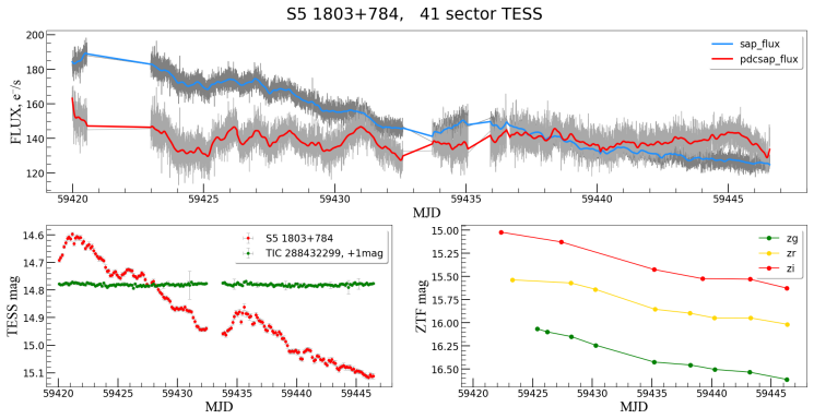
Summary. The manuscript proposes a new method for studying the evolution of the shortest characteristic variability timescales in long, uniformly sampled blazar light curves. The method slides through the light curve, starting from 20-point intervals and extending each interval until an interior maximum of the structure function (SF) is detected, then moves to the next interval. The authors apply this method to TESS SAP, PDCSAP, and full-frame aperture photometry of the blazar S5 1803+784, and compare the results with ZTF multiband photometry. They report a correlation between the structure-function maximum (or maximum brightness amplitude) and the characteristic time tau_v, and no correlation with the spectral index. The paper interprets these results as evidence for jet sub-components with different volumes and Doppler factors.

Significance. If the reported SFmax–tau_v correlation is genuine, the paper offers a simple, easily applicable method for tracing changes in the dominant variability timescale on hour-to-day scales, and it provides a unified physical interpretation of fast blazar variability through Doppler-boosted sub-components with different volumes. The paper is transparent about its principal single-process assumption in Section 4 and about the data-dependent smoothing choices, and the use of comparison-star aperture photometry is a practical improvement over raw TESS products. The interpretation is falsifiable in the sense that it predicts approximately achromatic short-timescale variability tied to the Doppler factor. However, the central quantitative claim is not yet established: the correlation is quoted without uncertainties, no null simulation of a single red-noise process is presented, and the significance test is model-dependent. The method is simple enough to simulate, so the required validation is within the scope of a revision.

major comments (4)

[Section 3 and Section 4.3] The headline SFmax–tau_v correlation may be a selection effect of the segmentation algorithm rather than a property of the source. The algorithm grows each interval from 20 points until an SF maximum is found, and for a red-noise process the structure function generally rises with lag; intervals that happen to be longer will therefore tend to have both larger tau_v and larger SFmax. The aperture-photometry correlation r=0.97 (and r=0.99 for the maximum amplitude) is reported without a p-value, confidence interval, or sample size, and no null simulation of a single stationary red-noise process is provided. I request a simulation study in which light curves with an ARIMA or power-law power spectral density are passed through the same segmentation algorithm, to show that the observed (SFmax, tau_v) relation is not reproduced by the selection procedure. This is load-bearing because the Doppler-factor interpretation in Section 6 rests on that correlation.
[Section 3] The significance test is partly self-referential. The ARIMA/ARMA models are fitted to each selected segment and then used to generate 1000 light curves whose SF peaks are compared with the observed peak of the same segment; the null distribution is therefore conditioned on the very data feature being tested. This test can indicate whether a peak is unusual under the fitted stationary model, but it does not validate the segmentation algorithm or the joint distribution of (SFmax, tau_v) that underlies the correlation claim. In addition, the paper notes that the model SF may have several maxima and that p may become negative, which shows that the reported quantity is a count of excess peaks rather than a proper probability. The authors should fit the noise model to data independent of the tested segment, and should use the simulated ensemble to construct a null distribution for the correlation statistic itself.
[Section 2.1 and Section 6] The choice of the 75-point Gaussian smoothing window is circular. The manuscript states in Section 6 that the window should be 'the smallest one for which the plateau on a plot SFmax(tau) is absent', and the plateau is judged on the same SFmax(tau) diagrams that are later used to claim the correlation. The paper tries windows from 5 to 125 points and multiple smoothing methods, and Section 4.2 reports that the SAP correlation appears with 75-point Gaussian smoothing but disappears with 125-point smoothing. The reported correlation is therefore conditional on a data-dependent choice made after inspecting the results. A sensitivity analysis across smoothing windows, or a pre-defined criterion for selecting the window that does not use the outcome of the correlation test, should be required.
[Section 4] The method relies on the explicit assumption, stated in Section 4, that at any moment a single variability process is acting and that it is later replaced by another process with a different tau_v. If the observed light curve is a superposition of simultaneously active processes, the sliding-window algorithm will force a single tau_v per interval and will create artificial segment boundaries and timescales. The paper acknowledges this assumption but does not test the method on simulated superpositions of two or more processes. Since the physical conclusion in Section 6 interprets the segmented intervals as real sub-components of the jet, this untested premise is load-bearing. A simulation with superposed variability processes is needed to show that the recovered tau_v values and interval breaks are meaningful.

minor comments (5)

[Equation (1)] In the structure-function definition, the second term inside the sum appears as X(tau) but should presumably be X(i); as printed, the formula is dimensionally incorrect and does not match the description of a lagged difference. Please correct this typographical error.
[Section 2.1] The text says 'data from 41 sectors' but the following sections refer to 'the 41st sector'; since one TESS sector is about 27 days and the quoted interval is about two months, the plural '41 sectors' appears to be a typo for 'sector 41'. Please clarify.
[Section 4.1 and Section 6] There are several language issues that should be corrected: 'This beak indicates' should be 'This break indicates'; 'is not inapplicable' should be 'is not applicable' or 'is inapplicable'; and the abstract phrase 'the radiation spectrum deflects slightly from the power-law' should be reworded (e.g., 'deviates slightly from a power law').
[Figure 3 caption] The caption phrase 'the points, for define of which data in three and two filters were used' is ungrammatical; please rephrase to explain which points use three filters and which use two.
[Section 4.3] The quantity labeled 'magvar' in Fig. 13 is not defined in the text; please define it explicitly as the maximum brightness change within each interval.

Circularity Check

0 steps flagged · score 0.0 of 10

No significant circularity: the SFmax–τv correlation is derived from the data and the physical interpretation is presented as an inference, not as the input of a fit.

full rationale

The paper's core empirical result—the SFmax–τv correlation—is computed directly from structure functions on detected intervals (Section 3, Figs. 12–13), not produced by fitting the Doppler model to the data. The ARIMA/ARMA significance test (Section 3) is a Monte Carlo null test for individual peaks; generating nulls from the same segment is standard practice and does not make the detected peak equivalent to the null model. The smoothing-window choice (Section 6: 'We propose to define this size as the smallest one for which the plateau on a plot SFmax(τ) is absent') is calibrated on the same data and is a legitimate selection-effect concern, but it is not load-bearing: the unsmoothed aperture-photometry analysis reproduces the correlation with r=0.97 and 0.99 (Section 4.3, Fig. 13), so the central correlation does not reduce to the smoothing choice. The Doppler-factor/sub-component explanation is imported from the authors' prior work (Refs. [22], [26]) and is presented as an expectation ('it is natural to expect indications of this variability mechanism'), not as a machine-checked theorem or uniqueness argument; it is used to interpret, not to derive, the observations. The paper also states its own limitations (the one-process assumption in Section 4 and the need for longer series for the α–τv anticorrelation in Section 4.3), and those weaken evidential strength without creating definitional circularity. No equation in the paper is shown to be equivalent to its own input by construction, and no fitted parameter is renamed as a prediction. Hence no significant circularity is found.

Assumptions & free parameters 6 free parameters · 5 assumptions · 1 invented entities

The method depends on several hand-picked analysis parameters and a strong single-process assumption. The physical interpretation introduces sub-components as an explanatory construct without independent evidence, and the significance test uses noise models fitted to the same data being tested.

free parameters (6)

SFmax threshold = 0.0009 (0.03 mag)
Ad hoc threshold in Section 3 to suppress noise peaks; controls which intervals are accepted.
Smoothing window size = 75 points (Gaussian) for 600 s data
Chosen in Section 4.1 as the smallest window without a 'plateau' at the SFmax threshold; the result disappears for 125 points.
Initial segment length = 20 data points
Starting window for the sliding search in Section 3.
Slope-test neighborhood = 3 SF points on each side
Used to decide whether a structure-function local maximum exists (Section 3).
Max gap allowance = 5 missing points
Data series split when gaps exceed 5 consecutive points (Section 2.1).
Aperture photometry co-add = 20 full-frame cuts
Number of TESS full-frame image cuts summed to reduce noise (Section 2.2).

assumptions (5)

domain assumption The maximum of the structure function marks the characteristic variability time.
Invoked throughout Section 3; a standard but model-dependent interpretation.
domain assumption At each epoch a single variability process dominates.
Stated explicitly in Section 4 as the principal assumption of the new method.
domain assumption ARIMA/ARMA models fitted to each segment describe the statistical noise.
Used in Section 3 to generate 1000 model light curves for significance testing.
domain assumption The optical spectrum follows a power law so that a spectral index alpha can be measured.
Used in Section 2.3 to derive spectral indices from ZTF photometry.
domain assumption TESS SAP and PDCSAP data have known instrumental systematics that can be handled by the described procedures.
Relied on throughout Section 2 to justify the analysis of both data types.

invented entities (1)

Jet sub-components with different volumes and Doppler factors
purpose: Explains the SFmax-tau correlation and missing spectral-index correlation
Introduced as a model interpretation in Sections 5 and 6; no direct observational handle such as a predicted time-variable polarization or multi-frequency signature is provided.

how reviews work

0 comments

Cite this review

Pith. "Pith review of A new method for studying the blazar variability on the shortest time scales and its application to S5 1803+784." pith.science (2026). https://pith.science/paper/IUHRGVPW

@misc{pith2026241118125,
  author       = {Pith},
  title        = {Pith review of: A new method for studying the blazar variability on the shortest time scales and its application to S5 1803+784},
  year         = {2026},
  howpublished = {\url{https://pith.science/paper/IUHRGVPW}},
  note         = {Machine review of arXiv:2411.18125}
}

read the original abstract

We propose a new method for investigating the evolution of the properties of the blazar brightness variability on timescales from a few hours to a few days. Its essence lies in detecting sequentially located time intervals along the entire light curve, within which it is possible to determine the characteristic time of variability using the structure function. We applied this method to a uniform data series lasting several days provided by the TESS mission for blazar S5 1803+784. Then, we analyzed the found time parameters of variability coupled with the data of B-, V-, R-, and I-photometric observations. A correlation was found between the amplitude and the characteristic time of variability. The relation of these values with the spectral index of radiation has not been revealed. We conclude that the variability on a short time scale is formed due to the different Doppler factors for having different volume parts of the optical emitting region. At the same time, the radiation spectrum deflects slightly from the power-law.

Figures

Figures reproduced from arXiv: 2411.18125 by the authors.

**Figure 2.** Cuts from TESS full-frame images. The objects are indicated at the top of each [PITH_FULL_IMAGE:figures/full_fig_p006_2.png] view at source ↗

**Figure 3.** Optical spectral index according to ZTF data from July 24 to September 20, [PITH_FULL_IMAGE:figures/full_fig_p007_3.png] view at source ↗

Figures from the paper (12 more)

**Figure 4.** Figure 4: Therefore, we did not use the Gaussian width in the study, and it did [PITH_FULL_IMAGE:figures/full_fig_p010_4.png]

**Figure 4.** Figure 4: Structure functions for a long continuous series of observations (on the left) [PITH_FULL_IMAGE:figures/full_fig_p011_4.png]

**Figure 5.** Figure 5: An illustration of the relation between SF [PITH_FULL_IMAGE:figures/full_fig_p013_5.png]

**Figure 6.** Figure 6: Distribution of significance levels for the found SF peaks for data with a time [PITH_FULL_IMAGE:figures/full_fig_p014_6.png]

**Figure 7.** Figure 7: An illustration of the relation between SF [PITH_FULL_IMAGE:figures/full_fig_p016_7.png]

**Figure 8.** Figure 8: Distribution of significance levels for the found SF peaks for data with a time [PITH_FULL_IMAGE:figures/full_fig_p017_8.png]

**Figure 9.** Figure 9: The relation of the interval duration with the characteristic time of variability [PITH_FULL_IMAGE:figures/full_fig_p017_9.png]

**Figure 10.** Figure 10: The relation of the interval duration with the characteristic time of variability [PITH_FULL_IMAGE:figures/full_fig_p018_10.png]

**Figure 11.** Figure 11: Evolution of the characteristic time of variability. Except for the point symbols, [PITH_FULL_IMAGE:figures/full_fig_p019_11.png]

**Figure 12.** Figure 12: The dependence of the maximum brightness change within the considered [PITH_FULL_IMAGE:figures/full_fig_p020_12.png]

**Figure 13.** Figure 13: The square of the average amplitude (on the left), the interval durations (in [PITH_FULL_IMAGE:figures/full_fig_p021_13.png]

**Figure 14.** Figure 14: Changing SFmax and τv over time. PDCSAP and SAP data are provided for the corresponding light curves smoothed by a Gaussian with a core of 75 points. but it is noteworthy that τv, obtained by different data types, agrees well. Comparing the change in τv ( [PITH_FULL_…

Discussion (0). Continue with ORCID to comment.

Reference graph

Works this paper leans on

30 extracted references · 30 canonical work pages

[1]

N. S. Kardashev, A. V. Alakoz, A. S. Andrianov, M. I. Artyukhov, W. Baan, V. E. Babyshkin, N. Bartel, O. S. Bayandina, I. E. Val’tts, P. A. Voitsik, A. Z. Vorobyov, C. Gwinn, J. L. Gomez, G. Giovannini, D. Jauncey, M. Johnson, H. Imai, Y. Y. Kovalev, S. E. Kurtz, M. M. Lisakov, A. P. Lobanov, V. A. Molodtsov, B. S. Novikov, A. V. Pogodin, M. V. Popov, A. ...

work page 2017
[2]

Plavin, Y.Y

A. Plavin, Y.Y. Kovalev, Y.A. Kovalev, S. Troitsky, Observational Evi- dence for the Origin of High-energy Neutrinos in Parsec-scale Nuclei of Radio-bright Active Galaxies , Astrophys. J., 894, 101 (2020)

work page 2020
[3]

V. A. Allakhverdyan, A. D. Avrorin, A. V. Avrorin, V. M. Aynutdi- nov, Z. Bardaˇ cov´ a, I. A. Belolaptikov, E. A. Bondarev, I. V. Borina, N. M. Budnev, V. A. Chadymov, A. S. Chepurnov, V. Y. Dik, G. V. Domogatsky, A. A. Doroshenko, R. Dvornick´ y, A. N. Dyachok, Zh- A. M. Dzhilkibaev, E. Eckerov´ a, T. V. Elzhov, L. Fajt, V. N. Fomin, 26 A. R. Gafarov, K...

work page 2024
[4]

Bhatta, J

G. Bhatta, J. R. Webb, H. Hollingsworth, S. Dhalla, A. Khanuja, R. Bachev, D. A. Blinov, M. B¨ ottcher, O. J. A. Bravo Calle, P. Calcidese, D. Capezzali, D. Carosati, R. Chigladze, A. Collins, J. M. Coloma, Y. Efimov, A. C. Gupta, S. -M. Hu, O. Kurtanidze, A. Lamerato, V. M. Larionov, C. -U. Lee, E. Lindfors, B. Murphy, K. Nilsson, J. M. Ohlert, A. Oksane...

work page 2013
[5]

Bhatta, L

G. Bhatta, L. Stawarz, M. Ostrowski, A. Markowitz, H. Akitaya, A. A. Arkharov, R. Bachev, E. Ben ´ ıtez, G. A. Borman, D. Carosati, A. D. Ca- son, R. Chanishvili, G. Damljanovic, S. Dhalla, A. Frasca, D. Hiriart, S. -M. Hu, R. Itoh, D. Jableka, S. Jorstad, M. D. Jovanovic, K. S. Kawa- bata, S. A. Klimanov, O. Kurtanidze, V. M. Larionov, D. Laurence, G. Le...

work page 2016
[6]

Edelson, R

R. Edelson, R. Mushotzky, S. Vaughan, J. Scargle, P. Gandhi, M. Malkan, W. Baumgartner, Kepler Observations of Rapid Optical Vari- ability in the BL Lacertae Object W2R1926+42 , Astrophys. J., 766, 16 (2013)

work page 2013
[7]

G. R. Ricker, J. N. Winn, R. Vanderspek, D. W. Latham, G. Bakos, J. L. Bean, Z. K. Berta-Thompson, T. M. Brown, L. Buchhave, N. R. Butler, R. P. Butler, W. J. Chaplin, D. Charbonneau, J. Christensen- Dalsgaard, M. Clampin, D. Deming, J. Doty, N. De Lee, C. Dressing, E. W. Dunham, M. Endl, F. Fressin, J. Ge, T. Henning, M. J. Holman, W. Howard, S. Ida, J. ...

work page 2015
[8]

C. M. Raiteri, M. Villata, D. Carosati, E. Ben ´ ıtez, D. O. Kurtanidze, A. C. Gupta, D. O. Mirzaqulov, F. D’Ammando, V. M. Larionov, T. Pursimo, J. A. Acosta-Pulido, G. V. Baida, B. Balmaverde, G. Bon- noli, G. A. Borman, M. I. Carnerero, W. -P. Chen, V. Dhiman, A. Di Maggio, S. A. Ehgamberdiev, D. Hiriart, G. N. Kimeridze, O. M. Kur- tanidze, C. S. Lin,...

work page 2021

Show all 30 references

[9]

C. M. Raiteri, M. Villata, V. M. Larionov, S. G. Jorstad, A. P. Marscher, Z. R. Weaver, J. A. Acosta-Pulido, I. Agudo, T. Andreeva, A. Arkharov, R. Bachev, E. Ben ´ ıtez, M. Berton, I. Bj¨ orklund, G. A. Borman, V. Bozhilov, M. I. Carnerero, D. Carosati, C. Casadio, W. P. Chen...

2021
[10]

Z. R. Weaver, K. E. Williamson, S. G. Jorstad, A. P. Marscher, V. M. Larionov, C. M. Raiteri, M. Villata, J. A. Acosta-Pulido, R. Bachev, G. V. Baida, T. J. Balonek, E. Ben ´ ıtez, G. A. Borman, V. Bozhilov, M. I. Carnerero, D. Carosati, W. P. Chen, G. Damljanovic, V. Dhiman, ...

2020
[11]

Kishore, A

S. Kishore, A. C. Gupta, P. J. Wiita, Rapid Optical Flares in the Blazar OJ 287 on Intraday Timescales with TESS , Astrophys. J., 960, 11 (2024)

2024
[12]

C. R. Lawrence, J. R. Zucker, A. C. S. Readhead, S. C. Unwin, T. J. Pearson, W. Xu, Optical Spectra of a Complete Sample of Radio Sources. I. The Spectra, Astrophys. J. Suppl., 107, 541 (1996)

1996
[13]

E. Kun, M. Karouzos,K. ´E. Gab´ anyi, S. Britzen, O. M. Kurtanidze, L. ´A. Gergely, Flaring radio lanterns along the ridge line: long-term 29 oscillatory motion in the jet of S5 1803+784 , Monthly Not. Roy. Astron. Soc., 478, 359–370 (2018)

2018
[14]

Nesci, S

R. Nesci, S. Cutini, C. Stanghellini, F. Martinelli, A. Maselli, V. M. Lipunov, V. Kornilov, R. R. Lopez, A. Siviero, M. Giroletti, M. Orienti, Multiwavelength flare observations of the blazar S5 1803+784 , Monthly Not. Roy. Astron. Soc., 502, 6177–6187 (2021)

2021
[15]

Priya, R

S. Priya, R. Prince, A. Agarwal, D. Bose, A. ¨Ozd¨ onmez, E. Ege, Multiwavelength temporal and spectral analysis of Blazar S5 1803+78 , Monthly Not. Roy. Astron. Soc., 513, 2239–2251 (2022)

2022
[16]

Carrasco, G

L. Carrasco, G. Escobedo, A. Porras,E. Recillas, L. Felix, A recent NIR Flare and similar amplitude fluctuations near maximum light of the blazar [HB89] 1803+784 , The Astronomer’s Telegram, 16344, 1 (2023)

2023
[17]

Agarwal, A

A. Agarwal, A. Pandey, A. ¨Ozd¨ onmez, E. Ege, A. Kumar Das, V. Karakulak, Characterizing the Optical Nature of the Blazar S5 1803+784 during Its 2020 Flare , Astrophys. J., 933, 42 (2022)

2022
[18]

J. M. Jenkins, J. D. Twicken, S. McCauliff, J. Campbell, D. Sanderfer, D. Lung, M. Mansouri-Samani, F. Girouard, P. Tenenbaum, T. Klaus, J. C. Smith, D. A. Caldwell, A. D. Chacon, C. Henze, C. Heiges, D. W. Latham, E. Morgan, D. Swade, S. Rinehart, R. Vanderspek, The TESS scie...

2016
[19]

K. G. Stassun, R. J. Oelkers, J. Pepper, M. Paegert, N. De Lee, G. Torres, D. W. Latham, S. Charpinet, C. D. Dressing, D. Huber, S. R. Kane, S. L´ epine, A. Mann, P. S. Muirhead, B. Rojas-Ayala, R. Silvotti, S. W. Fleming, A. Levine, P. Plavchan, The TESS Input Catalog and Can...

2018
[20]

E. C. Bellm, S. R. Kulkarni, M. J. Graham, R. Dekany, R. M. Smith, R. Riddle, F. J. Masci, G. Helou, T. A. Prince, S. M. Adams, C. Barbarino, T. Barlow, J. Bauer, R. Beck, J. Belicki, R. Biswas, N. Blagorodnova, D. Bodewits, B. Bolin, V. Brinnel, T. Brooke, B. Bue, M. Bulla, R...

2019
[21]

M. A. Gorbachev, M. S. Butuzova, S. V. Nazarov, A. V. Zhovtan, Ev- idence of jet-caused 12-year optical periodicity of blazar OJ 287 , As- troparticle Physics, 160, 102965 (2024)

2024
[22]

M. S. Butuzova, A geometrical interpretation for the properties of multi- band optical variability of the blazar S5 0716+714, Astroparticle Physics, 129, 102577 (2021)

2021
[23]

V. R. Amirkhanyan, BV RI observations of the radio source S5 0716+71, Astronomy Reports, 50, 273-288 (2006)

2006
[24]

J. H. Simonetti, J. M. Cordes, D. S. Heeschen, Flicker of extragalactic radio sources at two frequencies , Astrophys. J., 296, 46–59 (1985)

1985
[25]

Emmanoulopoulos, I

D. Emmanoulopoulos, I. M. McHardy, P. Uttley, On the use of structure functions to study blazar variability: caveats and problems, Monthly Not. Roy. Astron. Soc., 404, 931–946 (2010)

2010
[26]

M. A. Gorbachev, M. S. Butuzova, S. G. Sergeev, S. V. Nazarov, A. V. Zhovtan Long-term Multiband Optical Variability of Blazar S5 0716+714, Astrophys. J., 928, 86 (2022)

2022
[27]

Ghisellini, F

G. Ghisellini, F. Tavecchio, M. Chiaberge, Structured jets in TeV BL Lac objects and radiogalaxies. Implications for the observed properties , Astron. and Astrophys., 432, 401–410 (2005). 31

2005
[28]

Tavecchio, G

F. Tavecchio, G. Ghisellini, D. Guetta, Structured Jets in BL Lac Ob- jects: Efficient PeV Neutrino Factories? , Astrophys. J. Lett., 793, L18 (2014)

2014
[29]

M. L. Lister, M. F. Aller, H. D. Aller, D. C. Homan, K. I. Kellermann, Y. Y. Kovalev, A. B. Pushkarev, J. L. Richards, E. Ros, T. Savolainen, MOJA VE. X. Parsec-scale Jet Orientation Variations and Superluminal Motion in Active Galactic Nuclei , Astron. J., 146, 120 (2013)

2013
[30]

M. L. Lister, D. C. Homan, K. I. Kellermann, Y. Y. Kovalev, A. B. Pushkarev, E. Ros, T. Savolainen, Monitoring Of Jets in Active Galac- tic Nuclei with VLBA Experiments. XVIII. Kinematics and Inner Jet Evolution of Bright Radio-loud Active Galaxies , Astrophys. J., 923, 30 (2021). 32

2021

Pith tools

Reviewed August 12, 2026 · model on record in the stance chip above.

[1] [1]

N. S. Kardashev, A. V. Alakoz, A. S. Andrianov, M. I. Artyukhov, W. Baan, V. E. Babyshkin, N. Bartel, O. S. Bayandina, I. E. Val’tts, P. A. Voitsik, A. Z. Vorobyov, C. Gwinn, J. L. Gomez, G. Giovannini, D. Jauncey, M. Johnson, H. Imai, Y. Y. Kovalev, S. E. Kurtz, M. M. Lisakov, A. P. Lobanov, V. A. Molodtsov, B. S. Novikov, A. V. Pogodin, M. V. Popov, A. ...

work page 2017

[2] [2]

Plavin, Y.Y

A. Plavin, Y.Y. Kovalev, Y.A. Kovalev, S. Troitsky, Observational Evi- dence for the Origin of High-energy Neutrinos in Parsec-scale Nuclei of Radio-bright Active Galaxies , Astrophys. J., 894, 101 (2020)

work page 2020

[3] [3]

V. A. Allakhverdyan, A. D. Avrorin, A. V. Avrorin, V. M. Aynutdi- nov, Z. Bardaˇ cov´ a, I. A. Belolaptikov, E. A. Bondarev, I. V. Borina, N. M. Budnev, V. A. Chadymov, A. S. Chepurnov, V. Y. Dik, G. V. Domogatsky, A. A. Doroshenko, R. Dvornick´ y, A. N. Dyachok, Zh- A. M. Dzhilkibaev, E. Eckerov´ a, T. V. Elzhov, L. Fajt, V. N. Fomin, 26 A. R. Gafarov, K...

work page 2024

[4] [4]

Bhatta, J

G. Bhatta, J. R. Webb, H. Hollingsworth, S. Dhalla, A. Khanuja, R. Bachev, D. A. Blinov, M. B¨ ottcher, O. J. A. Bravo Calle, P. Calcidese, D. Capezzali, D. Carosati, R. Chigladze, A. Collins, J. M. Coloma, Y. Efimov, A. C. Gupta, S. -M. Hu, O. Kurtanidze, A. Lamerato, V. M. Larionov, C. -U. Lee, E. Lindfors, B. Murphy, K. Nilsson, J. M. Ohlert, A. Oksane...

work page 2013

[5] [5]

Bhatta, L

G. Bhatta, L. Stawarz, M. Ostrowski, A. Markowitz, H. Akitaya, A. A. Arkharov, R. Bachev, E. Ben ´ ıtez, G. A. Borman, D. Carosati, A. D. Ca- son, R. Chanishvili, G. Damljanovic, S. Dhalla, A. Frasca, D. Hiriart, S. -M. Hu, R. Itoh, D. Jableka, S. Jorstad, M. D. Jovanovic, K. S. Kawa- bata, S. A. Klimanov, O. Kurtanidze, V. M. Larionov, D. Laurence, G. Le...

work page 2016

[6] [6]

Edelson, R

R. Edelson, R. Mushotzky, S. Vaughan, J. Scargle, P. Gandhi, M. Malkan, W. Baumgartner, Kepler Observations of Rapid Optical Vari- ability in the BL Lacertae Object W2R1926+42 , Astrophys. J., 766, 16 (2013)

work page 2013

[7] [7]

G. R. Ricker, J. N. Winn, R. Vanderspek, D. W. Latham, G. Bakos, J. L. Bean, Z. K. Berta-Thompson, T. M. Brown, L. Buchhave, N. R. Butler, R. P. Butler, W. J. Chaplin, D. Charbonneau, J. Christensen- Dalsgaard, M. Clampin, D. Deming, J. Doty, N. De Lee, C. Dressing, E. W. Dunham, M. Endl, F. Fressin, J. Ge, T. Henning, M. J. Holman, W. Howard, S. Ida, J. ...

work page 2015

[8] [8]

C. M. Raiteri, M. Villata, D. Carosati, E. Ben ´ ıtez, D. O. Kurtanidze, A. C. Gupta, D. O. Mirzaqulov, F. D’Ammando, V. M. Larionov, T. Pursimo, J. A. Acosta-Pulido, G. V. Baida, B. Balmaverde, G. Bon- noli, G. A. Borman, M. I. Carnerero, W. -P. Chen, V. Dhiman, A. Di Maggio, S. A. Ehgamberdiev, D. Hiriart, G. N. Kimeridze, O. M. Kur- tanidze, C. S. Lin,...

work page 2021