REVIEW 4 major objections 4 minor 36 references
Derivative Estimation of Multivariate Functional Data
T0 review · 4 major / 4 minor · reviewed 2026-08-12 · deepseek-v4-flash
Pith's one-line read This paper extends functional principal component analysis to derivatives of multivariate functional data, proposing DMFPCA and DMKL, and reports that DMFPCA is the more accurate method for densely observed data.
desk verdict Solid multivariate extension of known univariate derivative PCA, but the simulations handicap DMKL and the abstract overclaims the DMFPCA advantage. read the letter →
The pith
A machine-rendered reading of the paper's core claim, the machinery that carries it, and where it could break.
The reading
What carries the argument
The load-bearing object is the derivative covariance operator $\Gamma_d$ with kernel $C_d(s,t)=E[\,\partial^d X(s)\,\partial^d X(t)^\top\,]$, together with identity (4), which equates its featurewise diagonal blocks to differentiated covariance surfaces, $\partial^d\partial^d C^{[p,p]}(s_p,t_p)=E[\,\partial^d X^{[p]}(s_p)\,\partial^d X^{[p]}(t_p)\,]$. This identity lets DMFPCA estimate the derivative covariance from smoothed versions of the observed curves without unstable numerical differentiation of individual trajectories. From the spectral decomposition of $\Gamma_d$ come the derivative multivariate functional principal components $\psi_{d,k}$ and scores $\rho_{d,k}$ that reconstruct derivatives through the multivariate Karhunen-Loève expansion; Happ and Greven's Proposition 5 supplies the bridge from per-feature eigencomponents to the joint multivariate ones, and the BLUP construction of Dai et al. predicts univariate scores from noisy discrete observations.
What would settle it
Run a simulation in which the true curves violate Assumption 1, for example estimating second derivatives from curves that are only once differentiable or that have jumps, and compare both methods against analytic derivatives; if DMFPCA's eigencomponents remain accurate despite the violation, the identity is not the load-bearing step, and if they degrade sharply the assumption is confirmed as the gatekeeper. In a setting with known true derivatives, a more direct check is to compare $\partial^d\partial^d$ of the estimated featurewise covariance with the empirical covariance of the true derivatives, since a systematic discrepancy would falsify equation (4) as the estimation route.
Extended reading notes
Core claim
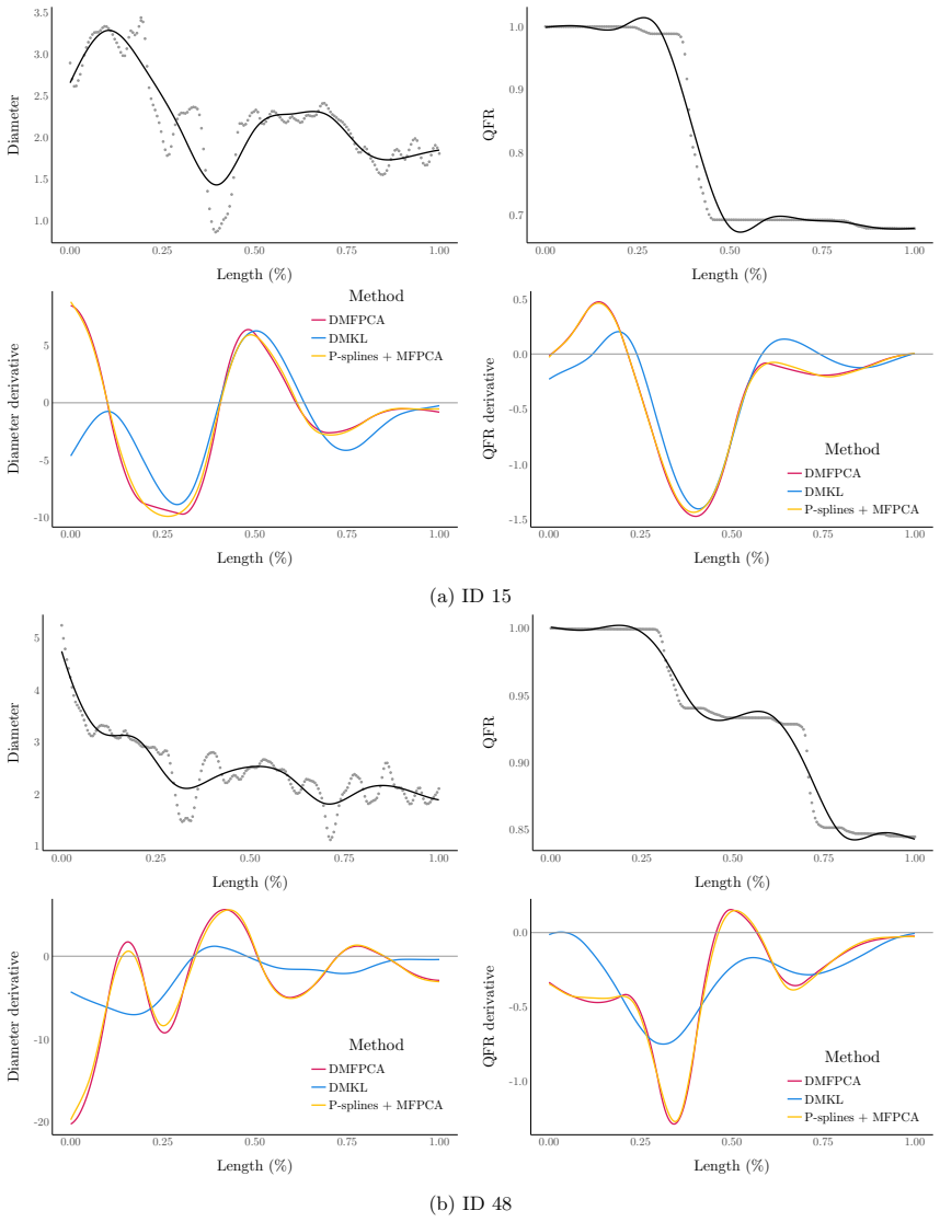
On the paper's own terms, the central discovery is that the derivative process $\partial^d X$ has its own multivariate Karhunen-Loève expansion, $\partial^d X(t)=\sum_{k=1}^\infty \rho_{d,k}\psi_{d,k}(t)$, and that the covariance operator of this derivative process can be reached without differentiating the raw curves: under Assumption 1, the $d$-th derivative of each featurewise covariance equals the covariance of the $d$-th derivatives, $\partial^d\partial^d C^{[p,p]}(s_p,t_p)=C_d^{[p,p]}(s_p,t_p)$. DMFPCA exploits this identity to estimate derivative eigencomponents from smoothed covariance surfaces and then links the univariate pieces into multivariate principal components, while DMKL instead differentiates the original eigenfunctions and reuses the original scores; because derivatives of eigenfunctions are not orthogonal, DMKL's expansion is suboptimal for a fixed truncation. The simulation study supports the claim that DMFPCA outperforms both DMKL and the direct P-splines-plus-MFPCA approach for dense data, and the angiogram application shows the derivative components and scores carrying information about where diameter narrows and QFR drops fastest.
Load-bearing premise
The argument stands on Assumption 1: the $d$-th derivative of the underlying process exists almost surely and lies in $H$, and the mixed partial derivative of each feature's covariance $\partial^d\partial^d C^{[p,p]}$ exists and is continuous, so that expectation and differentiation can be interchanged; if the observed curves are not smooth enough for these derivatives to exist, the estimated derivative components and scores are not well defined.
Editorial extensions
If this is right
- In dense, smooth settings, practitioners should expect DMFPCA to give the lowest errors in eigenfunctions, eigenvalues, and reconstructed derivatives, with average RMISE below 5% in the simulated no-noise and sigma=0.5 noise cases.
- DMKL remains a serviceable route for reconstructing derivatives even under high sparsity, with average RMISE below 15%, but with a fixed truncation it can badly miss later eigencomponents because the differentiated original eigenfunctions are not orthogonal.
- The direct approach of smoothing each curve, differentiating, and then running MFPCA is the safest fallback and the best of the three at medium sparsity, so the choice of method depends on sampling density.
- Derivative scores from DMFPCA and DMKL are usable as predictors in follow-up analyses, such as classifying coronary artery disease patterns into focal, serial, diffuse, and mixed types.
- In the coronary application, the methods locate the vessel position where diameter is narrowest and QFR is dropping fastest, information relevant to stent placement.
Reading between the lines
- The same covariance-differentiation template should extend to second and higher derivatives as long as Assumption 1 holds; a natural next experiment is to compare DMFPCA's second-derivative estimates against analytic derivatives on the paper's simulation family.
- DMFPCA's featurewise smoothing parameter is fixed in the simulation; adaptively choosing it per feature and per sampling density could close the gap to the direct approach in the medium-sparsity setting.
- Because derivative scores summarize dynamics rather than levels, they may separate CAD patterns better than scores from the original diameter and QFR curves; the paper shows score boxplots by pattern but does not run a formal classifier, so that is a testable extension.
- Identity (4) also opens a route to derivative estimation when curves from different features are observed on different grids, since the featurewise covariance derivatives can be estimated separately before the multivariate assembly step.
Editorial analysis
A structured set of objections, weighed in public.
Referee Report
Summary. The paper proposes two methods for estimating the principal components, scores, and reconstructed derivatives of multivariate functional data: DMFPCA, which differentiates the univariate covariance functions and then applies MFPCA, and DMKL, which differentiates the multivariate Karhunen-Loève expansion of the original data. The methods are compared with a direct approach (P-splines followed by MFPCA) in simulations covering dense, medium-sparse, and high-sparse settings, and applied to coronary angiogram data. The central claim is that DMFPCA outperforms the other methods, particularly for densely observed data.
Significance. If the claims hold, the paper fills a genuine gap by extending derivative-based FPCA to the multivariate setting. The two algorithms are clearly described and rely on standard theory (Kadota's differentiation theorem and Happ and Greven's relationship between univariate and multivariate FPCA). The simulation study is reasonably comprehensive and the application to coronary angiogram data is relevant, showing potential for clinical classification of coronary artery disease patterns. However, the central claim of DMFPCA's superiority is not fully established because of an asymmetric truncation in the DMKL comparison and because the medium-sparsity results contradict the abstract's general statement.
major comments (4)
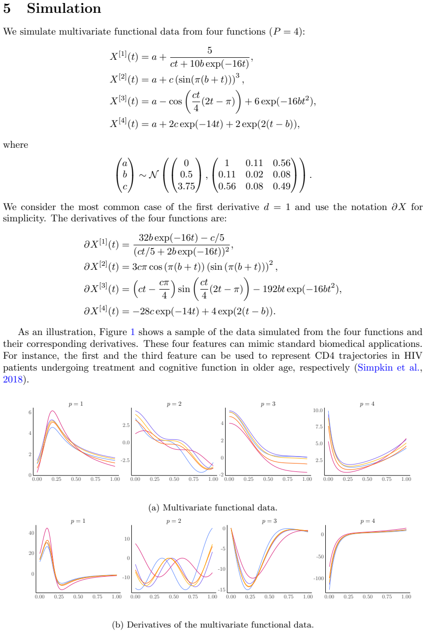
- [Section 5, Simulation (Figures 2–4)] The comparison between DMFPCA and DMKL is asymmetric with respect to truncation. In Algorithm 2, the initial MFPCA of the original curves is performed with K=3, so the intermediate derivative estimates are restricted to the span of derivatives of the first three MFPCs of X. This subspace is generically not the optimal three-dimensional subspace for the derivatives, and the large ISE/RE for DMKL's third component is a direct consequence of this truncation choice. The paper itself acknowledges this on page 8: 'Increasing the truncation number could enable DMKL to yield eigencomponents closer to the true result,' yet no such variant is run. The abstract's claim that 'DMFPCA outperforms DMKL' is therefore not supported by the reported simulations; it may reverse if DMKL is given a larger initial truncation (e.g., K'=10) before the final reduction to K=3. The authors should provide this sensitivity analysis or otherwise justify the truncation.
- [Section 5, medium sparsity setting] The central claim of DMFPCA's superiority is contradicted by the medium-sparsity results. The text on page 9 states: 'For medium sparsity case, DMFPCA yields slightly higher ISE than the P-splines + MFPCA method for all three eigenfunctions,' and Figure 4 shows that P-splines+MFPCA has the lowest RMISE (around 8%) compared with DMFPCA (around 10%). The abstract and the concluding discussion claim that 'DMFPCA outperforms DMKL and the direct approach, particularly for densely observed data,' but the only setting in which DMFPCA is consistently best is the dense case. The authors should either qualify the claim to 'for dense and high-sparsity settings' or provide an explanation for why medium sparsity is an exception, rather than making a blanket statement.
- [Sections 4.1 and 4.2, Algorithm details] The estimators used in the simulation are not fully specified, which compromises reproducibility and the comparability of the methods. In Algorithm 1 (DMFPCA), the estimation of ∂^d∂^d C^{[p,p]} is left to the reader, but the simulation text only mentions that 'we use P-splines with same smoothing parameter to estimate ∂^d∂^d C^{[p,p]} for both medium and high sparsity cases.' The actual smoothing parameter is not given. Similarly, in Algorithm 2 (DMKL), the derivative of the estimated eigenfunctions is stated as 'left to the reader,' but the simulation must have used a specific method (e.g., finite differences), which is not reported. Without these details, the numerical results cannot be reproduced, and differences between methods may be driven by implementation choices rather than the algorithms themselves.
- [Section 6, Application and Assumption 1] The application pre-smooths the raw coronary angiogram curves with P-splines before applying DMFPCA and DMKL. The theoretical framework in Assumption 1 requires the d-th derivative of the observed process to exist almost surely, but raw curves are irregular and noisy, so the derivatives are well-defined only for the smoothed curves. The paper does not discuss that the DMFPCs and scores estimated in Section 6 describe the smoothed process, not the raw measurement process. While pre-smoothing is a common practical device, the authors should explicitly state that the interpretation of the estimated components is conditional on the smoothing step and clarify how this relates to the theoretical assumptions.
minor comments (4)
- [Section 5, ISE definition] In the definition of ISE, the estimated eigenfunction is written as bψ^{(p)}_{d,k}(t_p), but elsewhere the notation is bψ^{[p]}_{d,k}; the parentheses appear to be a typo and the brackets are used consistently throughout the paper.
- [Section 5, Ground truth] The ground truth is obtained by applying MFPCA to the true derivatives and selecting K=3. It would be helpful to state the total variation explained by the first three components of the true derivative process (the text says '93%' but does not report the individual percentages), since this is the benchmark for the comparison.
- [Section 6, Figure 6 and 7 captions] The captions say 'plus (blue) and minus (purple) the estimated eigenfunctions,' which is ambiguous; it should read 'the estimated mean derivative functions (red), the mean derivative plus the eigenfunction (blue), and the mean derivative minus the eigenfunction (purple)' to make the interpretation clear.
- [Section 7, Discussion] The discussion repeats the claim that DMFPCA 'should be the preferred choice over the other two methods, particularly for practical applications,' which is too strong given the medium-sparsity results. The wording should be consistent with the qualified simulation findings.
Circularity Check
No significant circularity: the derivative eigencomponents and scores are estimated from independent definitions and external mathematical results, with no fitted parameter relabeled as a prediction.
full rationale
The paper's derivation chain is self-contained. The target objects (DMFPCs and DMFPC-scores) are defined as the eigencomponents of the derivative covariance operator Γ_d and the scores of the derivative process in its Karhunen-Loève expansion, and both algorithms estimate these quantities from the data without fitting a parameter that is then relabeled as the target. The simulation ground truth is obtained by applying MFPCA to the true derivatives, which is independent of the proposed estimators, so there is no fitted-input-called-prediction loop. The mathematical links invoked—Kadota's differentiation theorem, the interchange of expectation and differentiation in Equation (4), and the Happ-Greven univariate-to-multivariate relationship—are external results or standard derivations that do not reduce to the paper's own outputs. The only notable concern is that DMKL is simulated with an initial truncation of K=3 even though the paper itself states that increasing the truncation number could bring DMKL closer to the true result; that is an experimental fairness or correctness issue, not a circularity of the derivation. Self-citations to Golovkine et al. are used for supporting lemmas that are standard and not load-bearing in a circular sense. No circular step can be exhibited by quoting an equation that is identical to its own input by construction.
Assumptions & free parameters
free parameters (2)
- Truncation number K =
3 in simulation, 5 in application
- P-spline smoothing parameter =
0.1 in the application; 'same smoothing parameter' for simulation settings
assumptions (5)
- domain assumption Assumption 1: the d-th derivative of X exists almost surely and is in H; ∂^d∂^d C^{[p,p]} exists and is continuous.
- standard math Γ and Γ_d are compact positive operators on H, so the Hilbert-Schmidt spectral theory applies.
- domain assumption Interchange of expectation and differentiation in Eq. (4) under Assumption 1 and finite second moments.
- domain assumption The univariate-multivariate relationship of Happ and Greven (2018, Prop. 5) applies to the estimated derivative eigencomponents.
- domain assumption Sampling scheme: M and T are independent random variables; errors ε are i.i.d. with finite variance σ^2.
Cite this review
Pith. "Pith review of Derivative Estimation of Multivariate Functional Data." pith.science (2026). https://pith.science/paper/A7ZLYWZM
@misc{pith2026241118398,
  author       = {Pith},
  title        = {Pith review of: Derivative Estimation of Multivariate Functional Data},
  year         = {2026},
  howpublished = {\url{https://pith.science/paper/A7ZLYWZM}},
  note         = {Machine review of arXiv:2411.18398}
}
read the original abstract
Existing approaches for derivative estimation are restricted to univariate functional data. We propose two methods to estimate the principal components and scores for the derivatives of multivariate functional data. As a result, the derivatives can be reconstructed by a multivariate Karhunen-Lo\`eve expansion. The first approach is an extended version of multivariate functional principal component analysis (MFPCA) which incorporates the derivatives, referred to as derivative MFPCA (DMFPCA). The second approach is based on the derivation of multivariate Karhunen-Lo\`eve (DMKL) expansion. We compare the performance of the two proposed methods with a direct approach in simulations. The simulation results indicate that DMFPCA outperforms DMKL and the direct approach, particularly for densely observed data. We apply DMFPCA and DMKL methods to coronary angiogram data to recover derivatives of diameter and quantitative flow ratio. We obtain the multivariate functional principal components and scores of the derivatives, which can be used to classify patterns of coronary artery disease.
Figures


Figures from the paper (6 more)


Reference graph
Works this paper leans on
-
[1]
Biscaglia, S., Verardi, F. M., Tebaldi, M., Guiducci, V., Caglioni, S., Campana, R., Scala, A., Marrone, A., Pompei, G., Marchini, F., et al. (2023). Qfr-based virtual pci or conventional angiography to guide pci: the aqva trial. Cardiovascular Interventions , 16(7):783--794
work page 2023
-
[2]
Cao, J., Cai, J., and Wang, L. (2012). Estimating curves and derivatives with parametric penalized spline smoothing. Statistics and Computing , 22:1059--1067
work page 2012
-
[3]
Chiou, J.-M., Chen, Y.-T., and Yang, Y.-F. (2014). Multivariate functional principal component analysis: A normalization approach. Statistica Sinica , pages 1571--1596
work page 2014
-
[4]
Dai, X., M \"u ller, H.-G., and Tao, W. (2018). Derivative principal component analysis for representing the time dynamics of longitudinal and functional data. Statistica Sinica , 28(3):1583--1609
work page 2018
-
[5]
De Boor, C. (1972). On calculating with B -splines. Journal of Approximation Theory , 6(1):50--62
work page 1972
-
[6]
Eilers, P. H. and Marx, B. D. (2021). Practical smoothing: The joys of P-splines . Cambridge University Press
2021
-
[7]
Fan, J. and Gijbels, I. (1996). Local Polynomial Modelling and Its Applications: Monographs on Statistics and Applied Probability , volume 66. CRC Press
work page 1996
-
[8]
E., and Wand, M
Fan, J., Heckman, N. E., and Wand, M. P. (1995). Local polynomial kernel regression for generalized linear models and quasi-likelihood functions. Journal of the American Statistical Association , 90(429):141--150
1995
Show all 36 references
-
[9]
P., Press, W
Flannery, B. P., Press, W. H., Teukolsky, S. A., and Vetterling, W. T. (1992). Numerical recipes in C . Press Syndicate of the University of Cambridge, New York , 24(78):36
1992
-
[10]
and M \"u ller, H.-G
Gasser, T. and M \"u ller, H.-G. (1984). Estimating regression functions and their derivatives by the kernel method. Scandinavian Journal of Statistics , pages 171--185
1984
-
[11]
J., and Bargary, N
Golovkine, S., Gunning, E., Simpkin, A. J., and Bargary, N. (2023). On the use of the Gram matrix for multivariate functional principal components analysis
2023
-
[12]
Golovkine, S., Klutchnikoff, N., and Patilea, V. (2022). Clustering multivariate functional data using unsupervised binary trees. Computational Statistics & Data Analysis , 168:107376
2022
-
[13]
K., and Kneip, A
Grith, M., Wagner, H., H \"a rdle, W. K., and Kneip, A. (2018). Functional Principal Component Analysis for Derivatives of Multivariate Curves . Statistica Sinica , 28(4):2469--2496
2018
-
[14]
Hall, P., M \"u ller, H.-G., and Yao, F. (2009). Estimation of functional derivatives. The Annals of Statistics , 37(6A):3307--3329
2009
-
[15]
and Greven, S
Happ, C. and Greven, S. (2018). Multivariate functional principal component analysis for data observed on different (dimensional) domains. Journal of the American Statistical Association , 113(522):649--659
2018
-
[16]
A., Lee, D.-J., Rodr \' guez- \'A lvarez, M
Hern \'a ndez, M. A., Lee, D.-J., Rodr \' guez- \'A lvarez, M. X., and Durb \'a n, M. (2023). Derivative curve estimation in longitudinal studies using P -splines. Statistical Modelling , 23(5-6):424--440
2023
-
[17]
M., Hastie, T
James, G. M., Hastie, T. J., and Sugar, C. A. (2000). Principal component models for sparse functional data. Biometrika , 87(3):587--602
2000
-
[18]
Kadota, T. (1967). Differentiation of K arhunen- L o \`e ve expansion and application to optimum reception of sure signals in noise. IEEE Transactions on Information Theory , 13(2):255--260
1967
-
[19]
and Reimherr, M
Kokoszka, P. and Reimherr, M. (2017). Introduction to functional data analysis . Chapman and Hall/CRC
2017
-
[20]
Li, C., Xiao, L., and Luo, S. (2020). Fast covariance estimation for multivariate sparse functional data. Stat , 9(1):e245
2020
-
[21]
and M \"u ller, H.-G
Liu, B. and M \"u ller, H.-G. (2009). Estimating derivatives for samples of sparsely observed functions, with application to online auction dynamics. Journal of the American Statistical Association , 104(486):704--717
2009
-
[22]
Manteiga, W. G. and Vieu, P. (2007). Statistics for functional data. Computational Statistics & Data Analysis , 51(10):4788--4792
2007
-
[23]
u ller, H.-G., Stadtm \
M \"u ller, H.-G., Stadtm \"u ller, U., and Schmitt, T. (1987). Bandwidth choice and confidence intervals for derivatives of noisy data. Biometrika , 74(4):743--749
1987
-
[24]
Ramsay, J. O. (1982). When the data are functions. Psychometrika , 47:379--396
1982
-
[25]
Ramsay, J. O. and Dalzell, C. J. (1991). Some tools for functional data analysis. Journal of the Royal Statistical Society Series B: Statistical Methodology , 53(3):539--561
1991
-
[26]
Ramsay, J. O. and Silverman, B. W. (2002). Applied functional data analysis: methods and case studies . Springer
2002
-
[27]
Ramsay, J. O. and Silverman, B. W. (2005). Functional data analysis . Springer, New York, 2nd edition
2005
-
[28]
Rao, C. R. (1958). Some statistical methods for comparison of growth curves. Biometrics , 14(1):1--17
1958
-
[29]
and Simon, B
Reed, M. and Simon, B. (1980). Methods of Modern Mathematical Physics : Functional Analysis . Gulf Professional Publishing
1980
-
[30]
Silverman, B. W. (1996). Smoothed functional principal components analysis by choice of norm. The Annals of Statistics , 24(1):1--24
1996
-
[31]
J., Durban, M., Lawlor, D
Simpkin, A. J., Durban, M., Lawlor, D. A., MacDonald-Wallis, C., May, M. T., Metcalfe, C., and Tilling, K. (2018). Derivative estimation for longitudinal data analysis: examining features of blood pressure measured repeatedly during pregnancy. Statistics in Medicine , 37(19):2...
2018
-
[32]
Simpkin, A. J. and Newell, J. (2013). An additive penalty P -spline approach to derivative estimation. Computational Statistics & Data Analysis , 68:30--43
2013
-
[33]
Wang, S., Jank, W., and Shmueli, G. (2008). Explaining and forecasting online auction prices and their dynamics using functional data analysis. Journal of Business & Economic Statistics , 26(2):144--160
2008
-
[34]
Yao, F., M \"u ller, H.-G., and Wang, J.-L. (2005). Functional data analysis for sparse longitudinal data. Journal of the American Statistical Association , 100(470):577--590
2005
-
[35]
and Wolfe, D
Zhou, S. and Wolfe, D. A. (2000). On derivative estimation in spline regression. Statistica Sinica , pages 93--108
2000
-
[36]
Zhu, Y., Fezzi, S., Bargary, N., Ding, D., Scarsini, R., Lunardi, M., Mammone, C., Wagener, M., Mcinerney, A., Toth, G., et al. (2024). Validation of machine-learning angiography-derived physiological pattern of coronary artery disease. medRxiv , pages 2024--10
2024
Reviewed August 12, 2026 · model on record in the stance chip above.
Discussion (0). Continue with ORCID to comment.