REVIEW 3 major objections 5 minor 74 references
One-loop electron self-energy with accelerated partial-wave expansion in Coulomb gauge
T0 review · 3 major / 5 minor · reviewed 2026-08-12 · deepseek-v4-flash
Pith's one-line read The Coulomb gauge makes one-loop electron self-energy calculations work all the way down to hydrogen, without expansions in the nuclear binding strength.
desk verdict A careful, valuable extension of accelerated partial-wave methods to Coulomb gauge, but the 2S1/2 Z=10 discrepancy with Indelicato and Mohr is too large to dismiss as 'minor' and needs a real explanation before the headline accuracy claim is credible. read the letter →
The pith
A machine-rendered reading of the paper's core claim, the machinery that carries it, and where it could break.
The reading
What carries the argument
The central object is the partial-wave expansion of the many-potential Dirac-Coulomb Green function $G^{(2+)}$ inside the self-energy loop; its slow convergence and the tail extrapolation of its partial-wave terms limit numerical accuracy. The machinery is the potential-expansion decomposition of the self-energy into zero-, one-, and many-potential terms, together with a subtraction-and-readdition trick: an explicitly computable approximate Green function $G^{(2+)}_a$ that captures the slowest-converging part is subtracted from $G^{(2+)}$ in the partial-wave sum and re-added in closed form. The YPS scheme uses $G^{(2+)}_a=G^{(0)}(\varepsilon+\Omega)-G^{(0)}(\varepsilon)-\Omega\,\partial_\varepsilon G^{(0)}$ with $\Omega=2Z\alpha/(x_1+x_2)$; the SC scheme uses $G^{(2+)}_a=\frac12 V(x_1)\partial^2_\varepsilon G^{(0)} V(x_2)$. In the Coulomb gauge these manipulations are carried through with the transverse photon propagator split into $D_1$ and $D_2$ parts, and the resulting radial integrals are evaluated with Whittaker-function representations of the Coulomb-Dirac Green function.
What would settle it
Recompute the hydrogen $1s$ self-energy without the tail extrapolation—for instance, by summing partial waves explicitly to $|\kappa|\sim 10^4$ in multiprecision arithmetic, as was done in earlier benchmark calculations—and compare with the paper's value $F_{\rm SE}=10.3167935(7)$; a difference at the $10^{-7}$ level would invalidate the extrapolation-based uncertainty estimate.
Extended reading notes
Core claim
The paper establishes that previous low-$Z$ difficulties in self-energy calculations were in large part a gauge artifact. In the Feynman gauge, individual zero-, one-, and many-potential contributions contain spurious terms of order $\alpha(Z\alpha)^2$ that cancel only after summation, producing catastrophic cancellations as $Z\alpha$ shrinks; the physical result starts at order $\alpha(Z\alpha)^4$. Working in the Coulomb gauge removes these spurious contributions and simultaneously improves the convergence of the partial-wave expansion. Implementing the accelerated-convergence schemes of YPS (summing multiple commutators with an effective potential $\Omega=2Z\alpha/(x_1+x_2)$) and of SC (commuting two Coulomb potentials out of the Green function) in the Coulomb gauge, the authors compute the dimensionless self-energy function $F_{\rm SE}(Z\alpha)$ for $Z=1$ through 100 and principal quantum numbers through $n=5$. For hydrogen's $1s$ state they obtain $F_{\rm SE}=10.3167935(7)$, consistent with the earlier benchmark value $10.316793650(1)$, and they present the first direct all-order values for $D_{5/2}$, $F$, and $G$ states for $Z<60$.
Load-bearing premise
The quoted numerical results and their error bars rely on the assumption that the partial-wave tail is well described by a polynomial in $1/|\kappa|$, so that fitting the last few partial-wave terms and extrapolating to infinity yields the true remainder.
Editorial extensions
If this is right
- For hydrogen-like ions with $Z=1$ through roughly 10, the method delivers self-energy values with 2–7 more significant digits than previous all-order approaches for states beyond the low-$n$, low-$\ell$ set, enabling sharper comparisons with spectroscopic data.
- First direct all-order results for $D_{5/2}$, $F$, and $G$ states at $Z<60$ become available, providing benchmarks for the $Z\alpha$-expansion coefficients (such as $A_{60}$ and $A_{70}$) that enter these high-angular-momentum levels.
- The agreement with the benchmark hydrogen values provides an independent check of the theoretical input to the Rydberg constant determination.
- Because the Coulomb-gauge formulation is free of the low-$Z$ cancellations, the same subtraction machinery can be applied to the two-loop self-energy and vertex corrections in the low-$Z$ region, a direction the paper explicitly identifies as the next target.
Reading between the lines
- The same Coulomb-gauge acceleration approach should transfer to self-energy calculations with a finite nuclear size or with a screening potential, since the acceleration acts on the free-electron part of the Green function and does not depend on the specific bound-state potential; this would extend the method beyond the point-nucleus hydrogen-like ions treated here.
- For high-$\ell$ states the $Z$-dependence of $F_{\rm SE}(Z\alpha)$ is smooth, so interpolating the tabulated values would give accurate self-energy corrections at arbitrary $Z$ in the range 1–100 without recomputing each point.
- The improved low-$Z$ values can tighten tests of the $Z\alpha$-expansion, in particular pinning down the unknown $A_{70}$ coefficient, which the paper currently bounds only by a scale estimate of $0\pm 8A_{60}$.
- A comparison of YPS and SC results at fixed $Z$ for states where the two schemes differ by more than the quoted uncertainty would give a direct empirical check of the extrapolation error, since the two rely on different approximate Green functions.
Signed reviews
Editorial analysis
A structured set of objections, weighed in public.
Referee Report
Summary. The manuscript generalizes the potential-expansion approach for the one-loop electron self-energy to the general covariant gauge and the Coulomb gauge, and implements the YPS and Sapirstein–Cheng accelerated partial-wave convergence schemes in the Coulomb gauge. It presents numerical results for hydrogen-like ions in the range Z=1–100 for states up to n=5, including D5/2, F, and G states, and reports comparisons with Jentschura–Mohr, Mohr–Kim, and Indelicato–Mohr values. The central claims are that the Coulomb gauge avoids low-Z numerical cancellations, that the accelerated schemes give high accuracy down to Z=1, and that the approach is applicable to arbitrary excited states. Most comparisons agree with the literature at the quoted level, but the 2S1/2 Z=10 entry of Table III disagrees with the high-precision result of Ref. [19] by far more than the combined uncertainties, and the paper does not analyze this discrepancy.
Significance. If validated, this would be a significant methodological and numerical contribution: it provides an independent all-order cross-check of the Jentschura–Mohr hydrogen values, extends direct all-order self-energy calculations to D5/2, F, and G states for Z<60, and shows a practical accuracy gain from combining the Coulomb gauge with YPS/SC acceleration. The paper does not ship code, but the extended tables in the supplementary material are useful for benchmarks. However, the unresolved Table III discrepancy and the heuristic nature of the partial-wave extrapolation uncertainty prevent full confidence in the headline claim until those points are addressed.
major comments (3)
- [§IV, Table III (2S1/2 row, Z=10)] The value F(2S1/2, Z=10)=4.8944161(2) differs from the Indelicato–Mohr result 4.8944444(6) by 2.8×10^-5, roughly 45 times the combined quoted uncertainty. The text in §IV dismisses this as a 'minor discrepancy' without quantitative analysis. This is not a minor issue because the entry lies in the benchmark region (moderate Z, an excited state with nontrivial numerical cancellations) that is supposed to validate the method, and it is far outside the error bars of both calculations. Please provide a concrete explanation: either correct the present value, show with a controlled numerical experiment that the quoted uncertainty is underestimated, or demonstrate a specific reason to question the literature value.
- [§III, partial-wave extrapolation paragraph (Eq. (55))] The uncertainty of the final values is set by comparing extrapolations obtained when varying |κmax| by 20% and by choosing among fits of the form δE_|κ|=Σ c_l/|κ|^l. This procedure assumes that the asymptotic model Eq. (55) is an accurate representation of the tail; if the true tail contains state-dependent logarithmic or oscillatory terms, the extrapolated contribution can be biased by more than the estimated uncertainty. In view of the 2S1/2 Z=10 discrepancy, the paper should demonstrate with a known-benchmark state (for example, the 2P states with accurate literature values) that the extrapolated tail is stable under changes of (l0,l1), the number of fitted terms, and the |κmax| window, and that the quoted errors cover the resulting spread.
- [§IV, discussion of A70 (around Eq. (57))] The estimate A70=0±8A60 is calibrated by comparing the Zα expansion with the all-order results for the hydrogen 2P states. This tuned uncertainty is then used to assess whether the new all-order results for other states at Z=1 and Z=5 agree with the Zα-expansion predictions. The cross-check is therefore partially circular: agreement cannot be stronger than the calibration chosen for A70. Please either use an independent estimate of A70 (for example, from known higher-order coefficients or from a different data set) or formulate the low-Z comparisons without relying on this tuned uncertainty.
minor comments (5)
- [§IV] The statement that the Coulomb gauge is 'the optimal choice' is stronger than the evidence in Table I, which compares gauges for a single state (1s, Z=10) plus the hydrogen 1s case; a more precise phrasing would be 'advantageous for low-Z states tested here'.
- [§IV] The phrase 'arbitrary excited reference states' overstates the demonstrated scope; the results cover n≤5 and l≤4 for the listed states. Qualify this claim or provide results for higher-n/higher-l states.
- [§IV] The sentence 'with only minor discrepancies observed for the 1S and 2S states at Z=10' should be revised to reflect the quantitative analysis requested in the major comments; at present the statement is not supported by the numbers in Table III.
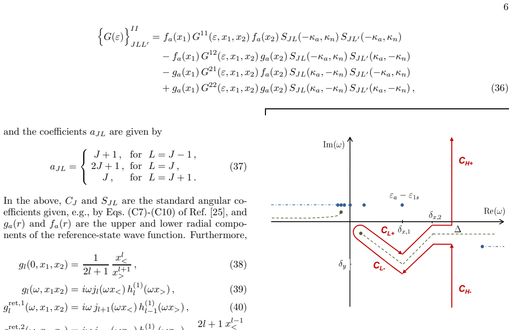
- [§III] The contour parameters δy, δx1, δx2 are chosen empirically; a sentence reporting the sensitivity of the final values to their variation would improve reproducibility.
- [Supplementary material] The reference to the supplementary material [54] still contains a placeholder URL; please insert the final link.
Circularity Check
No significant circularity; the numerical self-energy values are evaluated from established QED expressions and benchmarked externally against independent literature values.
full rationale
The derivation chain is self-contained. The zero-, one-, and many-potential terms are obtained by evaluating the standard unrenormalized self-energy expression (Eq. 1) with renormalized free-electron operators and Green functions; no target F(Zα) value is used as an input. The YPS and SC accelerated-convergence schemes from Refs. [30,31] are cited, but their content is restated in Eqs. (46) and (52), and they are used only to subtract and re-add an approximate Green function, so the final result does not depend on the accuracy of that approximation. The only self-cited inputs are method descriptions, not unverified claims, and the final values are compared with independent calculations by Jentschura and Mohr, Indelicato and Mohr, and Mohr and Kim across Z=1-40 and many states. The partial-wave tail extrapolation in Sec. III is a technical fit to polynomials in 1/|κ|, with uncertainty estimated by varying |κmax| by 20%; this fit does not encode the final energy values, which are dominated by explicit terms and anchored externally. The unresolved 2S1/2 Z=10 discrepancy with Ref. [19] is a validation and correctness concern, not a circularity, because the paper's own equations do not define the output in terms of the fit or of the cited method. No circular step is therefore identified.
Assumptions & free parameters
free parameters (3)
- Partial-wave extrapolation coefficients c_l =
Not reported; fitted per state to the last 4-5 partial-wave terms with (l0,l1) typically (3,4), (3,5), (3,6)
- A70 uncertainty coefficient (8) =
8
- Integration contour parameters delta_y, Delta, delta_x1, delta_x2 =
Chosen empirically, e.g. delta_y=(epsilon_a-epsilon_1s)/2 and Delta=Zalpha*epsilon_a for low Z
assumptions (4)
- standard math The renormalized potential-expansion decomposition into zero-, one-, and many-potential terms is valid.
- domain assumption The point-nucleus Coulomb potential is a sufficient model for the comparison.
- domain assumption The partial-wave tail follows the asymptotic 1/|kappa|^l form used for extrapolation.
- domain assumption Quadruple precision arithmetic is sufficient to control numerical cancellations at low Z.
Cite this review
Pith. "Pith review of One-loop electron self-energy with accelerated partial-wave expansion in Coulomb gauge." pith.science (2026). https://pith.science/paper/PSRERN2H
@misc{pith2026241119135,
  author       = {Pith},
  title        = {Pith review of: One-loop electron self-energy with accelerated partial-wave expansion in Coulomb gauge},
  year         = {2026},
  howpublished = {\url{https://pith.science/paper/PSRERN2H}},
  note         = {Machine review of arXiv:2411.19135}
}
abstract
Numerical calculations of the electron self-energy without any expansion in the binding nuclear field are required in order to match the rapidly advancing precision of experimental spectroscopy. For the lightest elements, particularly hydrogen, these computations are complicated by large numerical cancellations and the slow convergence of the partial-wave expansion. Methods with accelerated convergence of the partial-wave expansion have been recently put forward [V. A. Yerokhin, K. Pachucki, V. M. Shabaev, Phys. Rev. A 72, 042502 (2005); J. Sapirstein and K. T. Cheng, Phys. Rev. A 108, 042804 (2023)]. In our work we extend the accelerated-convergence methods to the previously hardly accessible region of nuclear charges $Z < 5$ and higher excited states.
Figures
Reference graph
Works this paper leans on
- [19]
-
[1]
R. Loetzsch, H. Beyer, L. Duval, U. Spillmann, D. Bana´ s, P. Dergham, F. Kr¨ oger, J. Glorius, R. Grisenti, M. Guerra, et al., Nature 625, 673 (2024)
work page 2024
-
[2]
P. Pf¨ afflein, G. Weber, S. Allgeier, Z. Andelkovic, S. Bernitt, A. I. Bondarev, A. Borovik, L. Duval, A. Fleischmann, O. Forstner, et al., arXiv preprint arXiv:2407.04166 (2024)
arXiv 2024
- [3]
-
[4]
S. Kraft-Bermuth, V. Andrianov, A. Bleile, A. Echler, P. Egelhof, P. Grabitz, S. Ilieva, O. Kiselev, C. Kilbourne, D. McCammon, et al., J. Phys. B 50, 055603 (2017)
work page 2017
- [5]
-
[6]
A. M. Desiderio and W. R. Johnson, Phys. Rev. A 3, 1267 (1971)
work page 1971
-
[7]
G. E. Brown, J. S. Langer, and G. W. Schaefer, Proc. R. Soc. London, Ser. A 251, 92 (1959)
work page 1959
Show all 74 references
-
[8]
P. J. Mohr, Ann. Phys. (NY) 88, 26 (1974)
1974
-
[9]
P. J. Mohr, Ann. Phys. (NY) 88, 52 (1974)
1974
-
[10]
P. J. Mohr, Phys. Rev. A 26, 2338 (1982)
1982
-
[11]
P. J. Mohr, Phys. Rev. A 46, 4421 (1992)
1992
-
[12]
U. D. Jentschura, P. J. Mohr, and G. Soff, Phys. Rev. Lett. 82, 53 (1999)
1999
-
[13]
U. D. Jentschura, P. J. Mohr, and G. Soff, Phys. Rev. A 63, 042512 (2001)
2001
-
[14]
U. D. Jentschura and P. J. Mohr, Phys. Rev. A 69, 064103 (2004)
2004
-
[15]
Indelicato and P
P. Indelicato and P. J. Mohr, Phys. Rev. A 46, 172 (1992)
1992
-
[16]
Persson, I
H. Persson, I. Lindgren, and S. Salomonson, Phys. Scr. T46, 125 (1993)
1993
-
[17]
H. M. Quiney and I. P. Grant, Phys. Scr. T 46 , 132 (1993)
1993
-
[18]
L. N. Labzowsky and I. A. Goidenko, J. Phys. B 30, 177 (1997)
1997
-
[20]
Zamastil and V
J. Zamastil and V. Patk´ oˇ s, Phys. Rev. A 86, 042514 (2012)
2012
-
[21]
N. J. Snyderman, Ann. Phys. (NY) 211, 43 (1991)
1991
-
[22]
S. A. Blundell and N. J. Snyderman, Phys. Rev. A 44, R1427 (1991)
1991
-
[23]
K. T. Cheng, W. R. Johnson, and J. Sapirstein, Phys. Rev. A 47, 1817 (1993)
1993
-
[24]
Mitrushenkov, L
A. Mitrushenkov, L. Labzowsky, I. Lindgren, H. Persson , and S. Salomonson, Phys. Lett. A200, 51 (1995)
1995
-
[25]
V. A. Yerokhin and V. M. Shabaev, Phys. Rev. A 60, 800 (1999)
1999
-
[26]
Persson, S
H. Persson, S. Salomonson, P. Sunnergren, and I. Lind- gren, Phys. Rev. Lett. 76, 204 (1996)
1996
-
[27]
S. A. Blundell, K. T. Cheng, and J. Sapirstein, Phys. Rev. A 55, 1857 (1997). 12
1997
-
[28]
V. A. Yerokhin, A. N. Artemyev, T. Beier, G. Plunien, V. M. Shabaev, and G. Soff, Phys. Rev. A 60, 3522 (1999)
1999
-
[29]
V. A. Yerokhin, Phys. Rev. A 62, 012508 (2000)
2000
-
[30]
V. A. Yerokhin, K. Pachucki, and V. M. Shabaev, Phys. Rev. A 72, 042502 (2005)
2005
-
[31]
Sapirstein and K
J. Sapirstein and K. T. Cheng, Phys. Rev. A 108, 042804 (2023)
2023
-
[32]
V. A. Yerokhin, Phys. Rev. A 83, 012507 (2011)
2011
-
[33]
V. A. Yerokhin, K. Pachucki, Z. Harman, and C. H. Kei- tel, Phys. Rev. Lett. 107, 043004 (2011)
2011
-
[34]
V. A. Yerokhin, K. Pachucki, M. Puchalski, C. H. Keitel, and Z. Harman, Phys. Rev. A 102, 022815 (2020)
2020
-
[35]
A. V. Malyshev, E. A. Prokhorchuk, and V. M. Shabaev, Phys. Rev. A 109, 062802 (2024)
2024
-
[36]
V. A. Yerokhin, Z. Harman, and C. H. Keitel, https://arxiv.org/abs/2411.12459, 2024
2024 arXiv
-
[37]
G. S. Adkins, Phys. Rev. D 8, 1814 (1983)
1983
-
[38]
G. S. Adkins, Phys. Rev. D 34, 2489 (1986)
1986
-
[39]
Hedendahl and J
D. Hedendahl and J. Holmberg, Phys. Rev. A 85, 012514 (2012)
2012
-
[40]
M. E. Rose, Relativistic Electron Theory , John Wiley & Sons, NY, 1961
1961
-
[41]
P. J. Mohr, G. Plunien, and G. Soff, Phys. Rep. 293, 227 (1998)
1998
-
[42]
V. A. Yerokhin and A. V. Maiorova, Symmetry 12, 800 (2020)
2020
-
[43]
J. B. Mann and W. R. Johnson, Phys. Rev. A 4, 41 (1971)
1971
-
[44]
V. A. Yerokhin, C. H. Keitel, and Z. Harman, Phys. Rev. A 104, 022814 (2021)
2021
-
[45]
P. J. Mohr and B. N. Taylor, Rev. Mod. Phys. 72, 351 (2000)
2000
-
[46]
V. A. Yerokhin, K. Pachucki, and V. Patk´ oˇ s, Ann. Phys. (Leipzig) 531, 1800324 (2019)
2019
-
[47]
Pachucki, Ann
K. Pachucki, Ann. Phys. (NY) 226, 1 (1993)
1993
-
[48]
Jentschura and K
U. Jentschura and K. Pachucki, Phys. Rev. A 54, 1853 (1996)
1996
-
[49]
Le Bigot, U
E.-O. Le Bigot, U. D. Jentschura, P. J. Mohr, P. Indeli- cato, and G. Soff, Phys. Rev. A 68, 042101 (2003)
2003
-
[50]
S. G. Karshenboim, Z. Phys. D 39, 109 (1997)
1997
-
[51]
Le Bigot, P
E.-O. Le Bigot, P. Indelicato, and P. J. Mohr, Phys. Rev. A 64, 052508 (2001)
2001
-
[52]
P. J. Mohr and Y.-K. Kim, Phys. Rev. A 45, 2727 (1992)
1992
-
[53]
Tiesinga, P
E. Tiesinga, P. J. Mohr, D. B. Newell, and B. N. Taylor, Rev. Mod. Phys. 93, 025010 (2021)
2021
-
[54]
See Supplemental Material at [URL will be inserted by publisher] for the extended tables of our numerical re- sults. Appendix A: Photon propagator The photon propagator has the simplest form in the Feynman (F) ga uge, where it is given by Dµν F (ω,⃗ x1,⃗ x2) = − ∫ d3k (2π)3 ei...
-
[55]
+ (1 −xs)[u⃗ p′2 + (1 −u)⃗ p2]. (E11) Integration over one of the Feynman parameters ( s) in the above formulas can be easily carried out analytically in terms of basic integrals J01, J11, J12,J22, where Jik = ∫ 1 0 ds si (1 +sZ)k , (E12) and Z comes from representing ∆ Z = ∆ ...
-
[56]
038 82 − 0
35 0 . 038 82 − 0. 177 80 − 0. 015 94 0 . 000 014 87 (1) − 0. 000 099 87 (5)
-
[57]
007 13 (35) − 0
∞ (extr.) 0 . 007 13 (35) − 0. 052 0 (7) − 0. 005 51 (18) 0 . 000 000 93 (3) − 0. 000 030 47 (15) Total 4 . 654 01 (35) 4 . 653 9 (7) 4 . 654 08 (18) 4 . 654 162 33 (3) 4 . 654 162 50 (16) Ref. [19] 4 . 654 161 9 (1) 17 TABLE II: Individual contributions to the one-loop self-e...
-
[58]
001 096 (3) 0
35 0 . 001 096 (3) 0 . 000 095 4 (6) 0 . 000 056 5 (6)
-
[59]
000 086 (2) 0
∞ (extr.) 0 . 000 086 (2) 0 . 000 012 8 (3) − 0. 000 002 1 (8) Total 10 . 316 793 (8) 10 . 316 793 5 (7) 10 . 316 794 0 (10) Ref. [13] 10 . 316 793 650 (1) 18 TABLE III: The one-loop electron self-energy correction for hyd rogen and hydrogen-like ions, in terms of F (Zα). Stat...
-
[60]
251 627 078 (1)a 4
316 793 650 (1)a 6. 251 627 078 (1)a 4. 654 161 9 (1)c 3. 246 255 7 (4)c 2. 135 228 4 (1)e 2S1/ 2 10. 546 825 0 (4) 6 . 484 860 2 (4) 4 . 894 416 1 (2) 3 . 506 647 70 (5) 2 . 454 829 06 (3)
-
[61]
484 860 42 (1)a 4
546 825 185 (5)a 6. 484 860 42 (1)a 4. 894 444 4 (6)c 3. 506 647 8 (2)c 2. 454 829 2 (7)e 3S1/ 2 10. 605 614 0 (2) 6 . 543 385 8 (2) 4 . 952 410 3 (4) 3 . 563 302 3 (2) 2 . 508 273 0 (1)
-
[62]
543 385 98 (5)b 4
605 614 22 (5)b 6. 543 385 98 (5)b 4. 952 4 (2)d 3. 563 3 (1)d 2. 508 3 (1)d 4S1/ 2 10. 629 388 (2) 6 . 566 758 7 (7) 4 . 974 919 5 (8) 3 . 583 402 7 (3) 2 . 521 506 2 (2)
-
[63]
566 758 8 (2)b 4
629 388 4 (2)b 6. 566 758 8 (2)b 4. 974 9 (4)d 3. 583 4 (1)d 2. 521 5 (1)d 5S1/ 2 10. 641 349 (2) 6 . 578 390 (3) 4 . 985 839 (1) 3 . 592 309 0 (4) 2 . 524 604 5 (7)
-
[64]
592 3 (2)d 2
985 8 (6)d 3. 592 3 (2)d 2. 524 6 (1)d 2P1/ 2 − 0. 126 395 (1) − 0. 122 775 (4) − 0. 114 851 (1) − 0. 092 519 2 (6) − 0. 031 049 9 (3) − 0. 126 396 37 (1)a − 0. 122 774 94 (1)a − 0. 114 852 (2)c − 0. 092 519 0 (1)c − 0. 031 050 0 (4)e 3P1/ 2 − 0. 115 458 1 (8) − 0. 111 259 (2)...
-
[65]
125 623 30(1)a 0
123 498 56 (1)a 0. 125 623 30(1)a 0. 130 350 7(3)c 0. 143 838 75 (4)c 0. 179 594 9 (4)e 3P3/ 2 0. 134 414 (2) 0 . 136 794 (2) 0 . 142 085 9 (3) 0 . 157 185 7 (4) 0 . 197 728 2 (6)
-
[66]
136 7 (2)f 0
134 413 (2)f 0. 136 7 (2)f 0. 142 1 (2)d 0. 157 2 (1)d 0. 197 7 (1)d 4P3/ 2 0. 139 439 (2) 0 . 141 909 (2) 0 . 147 395 (2) 0 . 163 046 0 (2) 0 . 205 168 0 (4)
-
[67]
141 8 (2)f 0
139 439 (2)f 0. 141 8 (2)f 0. 147 7 (4)d 0. 163 0 (1)d 0. 205 2 (1)d 5P3/ 2 0. 142 215 (5) 0 . 144 724 (3) 0 . 150 297 (1) 0 . 166 190 8 (2) 0 . 208 962 2 (4)
-
[68]
144 6 (3)f 0
142 215 (2)f 0. 144 6 (3)f 0. 150 2 (6)d 0. 166 2 (1)d 0. 208 9 (1)d 3D3/ 2 − 0. 043 019 (2) − 0. 042 927 (1) − 0. 042 708 (3) − 0. 042 020 (2) − 0. 039 617 8 (7) − 0. 043 0183 3 (2)f − 0. 042 929 (2)f − 0. 042 8 (2)d − 0. 042 0 (1)d − 0. 039 6 (1)d 4D3/ 2 − 0. 041 007 (3) − 0...
-
[69]
040 43 (1)f 0
040 316 18 (9)f 0. 040 43 (1)f 0. 040 73 (9)f 0. 041 7 (7)f 4D5/ 2 0. 042 329 (1) 0 . 042 460 (4) 0 . 042 801 (2) 0 . 043 959 2 (5) 0 . 047 931 7 (5)
-
[70]
042 46 (1)f 0
042 328 7 (1)f 0. 042 46 (1)f 0. 042 8 (1)f 0. 043 9 (8)f 5D5/ 2 0. 043 476 (2) 0 . 043 612 (6) 0 . 043 973 (2) 0 . 045 196 (2) 0 . 049 415 0 (2)
-
[71]
043 61 (1)f 0
043 475 6 (1)f 0. 043 61 (1)f 0. 044 0 (1)f 0. 045 1 (8)f 4F5/ 2 − 0. 021 498 (2) − 0. 021 480 (4) − 0. 021 438 (4) − 0. 021 309 (3) − 0. 020 920 (2) − 0. 021 497 019 (7)f − 0. 021 480 9 (9)f − 0. 021 441 (7)f − 0. 021 32 (6)f 5F5/ 2 − 0. 020 874 (2) − 0. 020 857 (5) − 0. 020 ...
-
[72]
020 192 (3)f 0
020 169 90 (2)f 0. 020 192 (3)f 0. 020 25 (2)f 0. 020 4 (2)f 5F7/ 2 0. 020 795 (2) 0 . 020 819 (6) 0 . 020 882 (9) 0 . 021 115 (3) 0 . 021 899 5 (4)
-
[73]
020 820 (3)f 0
020 794 73 (3)f 0. 020 820 (3)f 0. 020 89 (3)f 0. 021 1 (2)f 5G7/ 2 − 0. 012 861 (1) − 0. 012 859 (6) − 0. 012 846 (6) − 0. 012 805 (2) − 0. 012 695 (3) − 0. 012 859 159 (3)f − 0. 012 854 6 (3)f − 0. 012 843 (3)f − 0. 012 81 (2)f 5G9/ 2 0. 012 142 (1) 0 . 012 148 (4) 0 . 012 1...
-
[74]
012 1475 (9)f 0
012 140927 (8)f 0. 012 1475 (9)f 0. 012 165 (8)f 0. 012 23 (6)f a Jentschura and Mohr 2001 [13], b Jentschura 2004 [14], c Indelicato and Mohr 1998 [19], d Mohr and Kim 1992 [52], e Mohr 1992 [11], f Zα expansion. 19 TABLE IV: The one-loop electron self-energy correction for n...
2001
Reviewed August 12, 2026 · model on record in the stance chip above.
Discussion (0). Continue with ORCID to comment.